24. Stochastic Processes
24.1 Introduction
A stochastic process \(\{ X_t : t \in T \}\) is a collection of random variables. We shall sometimes write \(X(t)\) instead of \(X_t\). The variables \(X_t\) take values in some set \(\mathcal{X}\) called the state space. The set \(T\) is called the index set and for our purposes can be thought of as time. The index set can be discrete, \(T = \{0, 1, 2, \dots \}\) or continuous \(T = [0, \infty)\) depending on the application.
Recall that if \(X_1, \dots, X_n\) are random variables then we can write the joint density as
\[ f(x_1, \dots, x_n) = f(x_1) f(x_2 | x_1) \dots f(x_n | x_1, \dots, x_{n-1}) = \prod_{i=1}^n f(x_i | \text{past}_i) \]
where \(\text{past}_i\) refers to all variables before \(X_i\).
24.2 Markov Chains
The process \(\{ X_n : n \in T \}\) is a Markov Chain if
\[ \mathbb{P}(X_n = x | X_0, \dots, X_{n-1}) = \mathbb{P}(X_n = x | X_{n-1})\]
for all \(n\) and for all \(x \in \mathcal{X}\).
For a Markov chain, the joint density function can be written as
\[ f(x_1, \dots, x_n) = f(x_1) f(x_2 | x_1) f(x_3 | x_2) \dots f(x_n | x_{n - 1}) \]
A Markov chain can be represented by the following DAG:
\[ X_1 \longrightarrow X_2 \longrightarrow X_3 \longrightarrow \cdots \longrightarrow X_n \longrightarrow \cdots \]
Each variable has a single parent, namely, the previous observation.
The theory of Markov chains is very rich and complex. Our goal is to answer the following questions:
When does a Markov chain “settle down” into some sort of equilibrium?
How do we estimate the parameters of a Markov chain?
How can we construct Markov chains that converge to a given equilibrium and why would we want to do that?
Questions 1 and 2 will be approached this chapter, question 3 in the next chapter.
import numpy as np

def generate_random_walk(n, seed=None):
    if seed is not None:
        np.random.seed(seed)

    X = np.empty(n)
    X[0] = 0
    for i in range(1, n):
        X[i] = X[i - 1] + np.random.uniform(low=-1, high=1)

    return X

def generate_random_walk_bound(n, drift=-0.4, min_value=-10, seed=None):
    if seed is not None:
        np.random.seed(seed)

    X = np.empty(n)
    X[0] = 0
    for i in range(1, n):
        X[i] = max(X[i - 1] + drift, min_value) + np.random.uniform(low=-1, high=1)

    return X
import matplotlib.pyplot as plt
%matplotlib inline
plt.figure(figsize=(12, 8))
A = generate_random_walk(1000, seed=0)
B = generate_random_walk_bound(1000, drift=-1, seed=0)
ax = plt.subplot(2, 1, 1)
ax.plot(np.arange(0, len(A)), A)
ax.set_title('Does not settle into equilibrium')
ax = plt.subplot(2, 1, 2)
ax.plot(np.arange(0, len(B)), B)
ax.set_title('Does settle into equilibrium')
plt.tight_layout()
plt.show()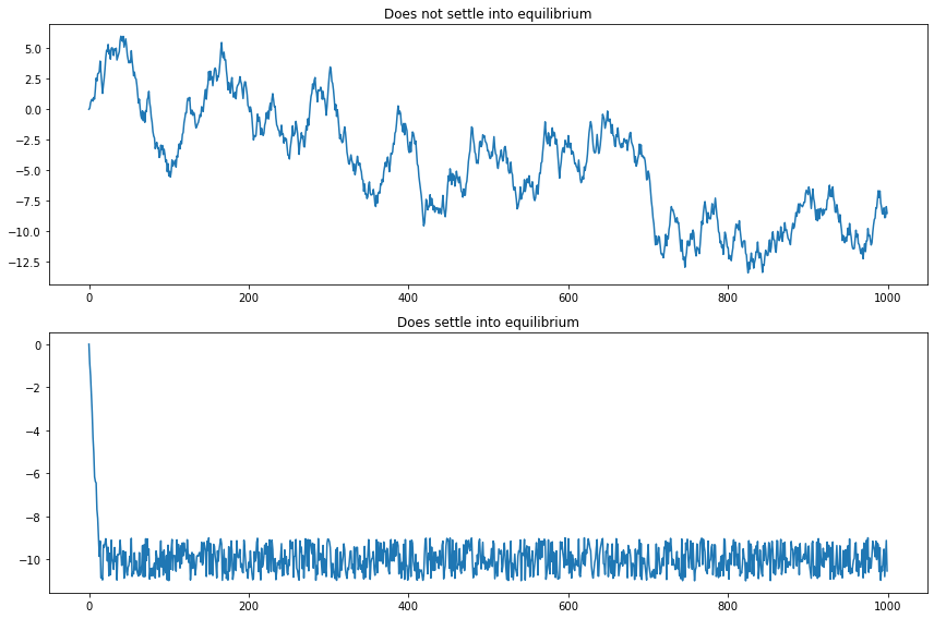
png
Transition Probabilities
The key quantities of a Markov chain are the probabilities of jumping from one state into another state.
We call
\[ \mathbb{P}(X_{n+1} = j | X_n = i) \]
the transition probabilities. If the transition probabilities do not change with time, we say the chain is homogeneous. In this case we define \(p_{ij} = \mathbb{P}(X_{n+1} = j | X_n = i)\). The matrix \(P\) whose \((i, j)\) element is \(p_{ij}\) is called the transition matrix.
We will only consider homogeneous chains. Notice how each \(P\) has two properties: (i) \(p_{ij} \geq 0\) and (ii) \(\sum_i p_{ij} = 1\). Each row is a probability mass function. A matrix with these properties is called a stochastic matrix.
Let
\[ p_{ij}(n) = \mathbb{P}(X_{m + n} = j | X_{m} = i) \]
be the probability of going from state \(i\) to state \(j\) in \(n\) steps. Let \(P_n\) be the matrix whose \((i, j)\) element is \(p_{ij}(n)\). These are called the \(n\)-step transition probabilities.
Theorem 24.9 (The Chapman-Kolmogorov equations). The \(n\)-step probabilities satisfy
\[ p_{ij}(m + n) = \sum_k p_{ik}(m) p_{kj}(n) \]
Proof. Recall that, in general,
\[ \mathbb{P}(X = x, Y = y) = \mathbb{P}(X = x) \mathbb{P}(Y = y | X = x) \]
This fact is true when conditioned in another variable,
\[ \mathbb{P}(X = x, Y = y | Z = z) = \mathbb{P}(X = x | Z = z) \mathbb{P}(Y = y | X = x, Z = z) \]
Also, recall the law of total probability:
\[ \mathbb{P}(X = x) = \sum_y \mathbb{P}(X = x, Y = y) \]
Using these facts and the Markov property we have:
\[ \begin{align} p_{ij}(m + n) &= \mathbb{P}(X_{m + n} = j | X_0 = i) \\ &= \sum_k \mathbb{P}(X_{m + n} = j, X_m = k | X_0 = i) \\ &= \sum_k \mathbb{P}(X_{m + n} = j | X_m = k, X_0 = i) \mathbb{P}(X_m = k | X_0 = i) \\ &= \sum_k \mathbb{P}(X_{m + n} = j | X_m = k) \mathbb{P}(X_m = k | X_0 = i) \\ &= \sum_k p_{ik}(m) p_{kj}(n) \end{align} \]
Note that this definition is equivalent to matrix multiplication; hence we have shown that
\[ P_{m + n} = P_m P_n \]
By definition, \(P_1 = P\). Using the above theorem, we get
\[ P_n = P^n \equiv \underbrace{P \times P \times \cdots \times P}_{\text{multiply matrix } n \text{ times}} \]
Let \(\mu_n = (\mu_n(1), \dots, \mu_n(N))\) be a row vector where
\[ \mu_n(i) = \mathbb{P}(X_n = i) \]
is the marginal probability that the chain is in state \(i\) at time \(n\). In particular, \(\mu_0\) is called the initial distribution. To simulate a Markov chain, all you need to know is \(\mu_0\) and \(P\). The simulation would look like this:
- Draw \(X_0 \sim \mu_0\). Thus, \(\mathbb{P}(X_0 = i) = \mu_0(i)\).
- Suppose the outcome of step 1 is \(i\). Draw \(X_1 \sim P\). In other words, \(\mathbb{P}(X_1 = j | X_0 = i) = p_{ij}\).
- Suppose the outcome of step 2 is \(j\). Draw \(X_2 \sim P\). In other words, \(\mathbb{P}(X_2 = k | X_1 = j) = p_{jk}\).
and so on.
It might be difficult to understand the meaning of \(\mu_n\). Imagine simulating the chain many times. Collect all of the outcomes at time \(n\) from all the chains. This histogram would look approximately like \(\mu_n\). A consequence of the previous theorem is the following:
Lemma 24.10. The marginal probabilities are given by
\[ \mu_n = \mu_0 P^n \]
Proof.
\[ \mu_n(j) = \mathbb{P}(X_n = j) = \sum_i \mathbb{P}(X_n = j | X_0 = i) \mathbb{P}(X_0 = i) = \sum_i \mu_0(i) p_{ij}(n) = \mu_0 P^n \]
Summary
- Transition matrix: \(P(i, j) = \mathbb{P}(X_{n+1} = j | X_n = i)\)
- \(n\)-step matrix: \(P_n(i, j) = \mathbb{P}(X_{m+n} = j | X_m = i)\)
- \(P_n = P^n\)
- Marginal probabilities: \(\mu_n(i) = \mathbb{P}(X_n = i)\)
- \(\mu_n = \mu_0 P^n\)
States
The states of a Markov chain can be classified according to various properties.
We say that \(i\) reaches \(j\) (or \(j\) is accessible from \(i\)) if \(p_{ij}(n) > 0\) for some \(n\), and we write \(i \rightarrow j\). If \(i \rightarrow j\) and \(j \rightarrow i\) then we write \(i \leftrightarrow j\) and we say that \(i\) and \(j\) communicate.
Theorem 24.12. The communication relation satisfies the following properties:
- \(i \leftrightarrow i\).
- If \(i \leftrightarrow j\) then \(j \leftrightarrow i\).
- If \(i \leftrightarrow j\) and \(j \leftrightarrow k\) then \(i \leftrightarrow k\).
- The set of states \(\mathcal{X}\) can be written as a disjoint union of classes \(\mathcal{X} = \mathcal{X}_1 \cup \mathcal{X}_2 \cup \cdots\) where two states \(i\) and \(j\) communicate with each other if and only if they are in the same class.
If all states communicate with each other then the chain is called irreducible. A set of states is closed if once you enter that set states you never leave. A closet set consisting of a single state is called an absorbing state.
Suppose we start a chain in state \(i\). Will the chain ever return to state \(i\)? If so, that state is called persistent or recurrent.
State \(i\) is recurrent or persistent if
\[ \mathbb{P}(X_n = i \text{ for some } n \geq 1 | X_0 = i) = 1 \]
Otherwise, state \(i\) is transient.
Theorem 24.15. A state \(i\) is recurrent if and only if
\[ \sum_n p_{ii}(n) = \infty \]
A state \(i\) is transient if and only if
\[ \sum_n p_{ii}(n) < \infty \]
Proof. Define
\[ I_n = \begin{cases} 1 & \text{if } X_n = i \\ 0 & \text{if } X_n \neq i \end{cases} \]
The number of times that the chain is in state \(i\) is \(Y = \sum_{n=0}^\infty I_n\). The mean of \(Y\), given that the chain starts in state \(i\), is
\[ \begin{align} \mathbb{E}(Y | X_0 = i) &= \sum_{n=0}^\infty \mathbb{E}(I_n | X_0 = i) \\ &= \sum_{n=0}^\infty \mathbb{P}(X_n = i | X_0 = i) \\ &= \sum_{n=0}^\infty p_{ii}(n) \end{align} \]
Define \(a_i = \mathbb{P}(X_n = i \text{ for some } n \geq 1 | X_0 = i)\). If \(i\) is recurrent, \(a_i = 1\). Thus, the chain will eventually return to \(i\). Once it does, we argue again that since \(a_i = 1\), the chain will return to state \(i\) again. By repeating this argument, we conclude that \(\mathbb{E}(Y | X_0 = i) = \infty\).
If \(i\) is transient, then \(a_i < 1\). When the chain is in state \(i\), there is a probability \(1 - a_i > 0\) that it will never return to state \(i\). Thus, the probability that the chain is in state \(i\) exactly \(n\) times is \(a_i^{n - 1}(1 - a_i)\). This is a geometric distribution that has finite mean.
Theorem 24.16. Facts about recurrence:
- If a state \(i\) is recurrent and \(i \leftrightarrow j\) then \(j\) is recurrent.
- If a state \(i\) is transient and \(i \leftrightarrow j\) then \(j\) is transient.
- A finite Markov chain must have at least one recurrent state.
- The states of a finite, irreducible Markov chain are all recurrent.
Theorem 24.17 (Decomposition Theorem). The state space \(\mathcal{X}\) can be written as the disjoint union
\[ \mathcal{X} = \mathcal{X}_{T} \cup \mathcal{X}_{1} \cup \mathcal{X}_{2} \cup \cdots \]
where the \(\mathcal{X}_T\) are the transient states and each \(\mathcal{X}_i\) is a closed, irreducible set of recurrent states.
Convergence of Markov Chains
Suppose that \(X_0 = i\). Define the recurrence time
\[ T_{ij} = \min \{ n > 0 : X_n = j \} \]
assuming \(X_n\) ever returns to the state \(i\), otherwise define \(T_{ij} = \infty\). The mean recurrence time of a recurrent state \(i\) is
\[ m_i = \mathbb{E}(T_{ii}) = \sum_n n f_{ii}(n) \]
where
\[ f_{ij}(n) = \mathbb{P}(X_1 \neq j, X_2 \neq j, \dots, X_{n-1} \neq j, X_n = j | X_0 = i) \]
A recurrent state is null if \(m_i = \infty\), otherwise it is called non-null or positive.
Lemma 24.18. If a state is null and recurrent, then \(p_{ii}^n \rightarrow 0\).
Lemma 24.19. In a finite state Markov chain, all recurrent states are positive.
Consider a three state chain with transition matrix
\[ \begin{bmatrix} 0 & 1 & 0 \\ 0 & 0 & 1 \\ 1 & 0 & 0 \end{bmatrix} \]
Suppose we start the chain in state 1. Then we will be in state 3 at times \(3, 6, 9, \dots\). This is an example of a periodic chain. Formally, the period of state \(i\) is \(d\) is \(p_{ii}(n) = 0\) whenever \(n\) is not divisible by \(d\) and \(d\) is the largest integer with this property. Thus, \(d = \text{gcd} \{ n : p_{ii}(n) > 0 \}\), where gcd means “greatest common divisor.” State \(i\) is periodic if \(d(i) > 1\) and aperiodic if \(d(i) = 1\).
Lemma 24.20. If a state \(i\) has period \(d\) and \(i \leftrightarrow j\) then \(j\) has period \(d\).
A state is ergodic if it is recurrent, non-null and aperiodic. A chain is ergodic if all its states are ergodic.
Let \(\pi = (\pi_i : i \in \mathcal{X})\) be a vector of non-negative numbers that sum to one. Thus \(\pi\) can be thought of as a probability mass function.
We say that \(\pi\) is a stationary (or invariant) distribution if \(\pi = \pi P\).
Here is the intuition. Draw \(X_0\) from distribution \(\pi\) and suppose that \(\pi\) is a stationary distribution. Now draw \(X_1\) according to the transition probability of the chain. The distribution of \(X_1\) is then \(\mu_1 = \mu_0 P = \pi P = \pi\). Continuing this way, the distribution of \(X_n\) is \(\mu_n = \mu_0 P^n = \pi P^n = \pi\). In other words: if at any time the chain has distribution \(\pi\), then it will continue to have distribution \(\pi\) forever.
We say that a chain has limiting distribution if
\[ P^n \rightarrow \begin{bmatrix} \pi \\ \pi \\ \vdots \\ \pi \end{bmatrix}\]
for some \(\pi\). In other words, \(\pi_j = \lim_{n \rightarrow \infty} P_{ij}^n\) exists and is independent of \(i\).
Theorem 24.24. An irreducible, ergodic Markov chain has a unique stationary distribution \(\pi\). The limiting distribution exists and is equal to \(\pi\). If \(g\) is any bounded function, then, with probabiity 1,
\[ \lim_{N \rightarrow \infty} \frac{1}{N} \sum_{n=1}^N g(X_n) = \mathbb{E}_\pi(g) \equiv \sum_j g(j) \pi_j \]
The last statement of the theorem is the law of large numbers for Markov chains. It says that sample averages converge to their expectations. Finally, there is a special condition which will be useful later. We say that \(\pi\) satisfies detailed balance if
\[ \pi_i p_{ij} = p_{ji} \pi_j \]
Detailed balance guarantees that \(\pi\) is a stationary distribution.
Theorem 24.25. If \(\pi\) satisfies detailed balance then \(\pi\) is a stationary distribution.
Proof. We need to show that \(\pi P = \pi\). The \(j\)-th element of \(\pi P\) is \(\sum_i \pi_i p_{ij} = \sum_i p_{ji}\pi_j = \pi_j \sum_i p_{ji} = \pi_j\).
The importance of detailed balance will become clear when we discuss Markov chain Monte Carlo methods.
Warning: Just because a chain has a stationary distribution does not mean it converges.
Inference for Markov Chains
Consider a chain with finite state space $ = { 1, 2, , N } $. Suppose we observe \(n\) observations \(X_1, \dots, X_n\) from this chain. The unknown parameters of a Markov chain are the initial probabilities \(\mu_0 = (\mu_0(1), \mu_0(2), \dots)\) and the elements of the transition matrix \(P\). Each row of \(P\) is a multinomial distribution, so we are essentially estimating \(N\) distributions (plus the initial probabilities). Let \(n_{ij}\) be the observed number of transitions from state \(i\) to state \(j\). The likelihood function is
\[ \mathcal{L}(\mu_0, P) = \mu_0(x_0) \prod_{r=1}^n p_{X_{r - 1}, X_r} = \mu_0(x_0) \prod_{i=1}^N \prod_{j=1}^N p_{ij}^{n_{ij}} \]
There is only one observation on \(\mu_0\) so we can’t estimate that. Rather, we focus on estimating \(P\). The MLE is obtained by maximizing the likelihood subject to the constraint that the elements are non-negative and the rows sum to 1. The solution is
\[ \hat{p}_{ij} = \frac{n_{ij}}{n_i} \]
where \(n_i = \sum_{j=1}^N n_{ij}\). Here we are assuming that \(n_i > 0\). If not, we set \(\hat{p}_{ij} = 0\) by convention.
Theorem 24.30 (Consistency and Asymptotic Normality of the MLE). Assume that the chain is ergodic. Let \(\hat{p}_{ij}(n)\) denote the MLE after \(n\) observations. Then \(\hat{p}_{ij}(n) \xrightarrow{\text{P}} p_{ij}\). Also,
\[ \left[ \sqrt{N_i(n)} (\hat{p}_{ij} - p_{ij}) \right] \leadsto N(0, \Sigma) \]
where the left hand side is a matrix, $ N_i(n) = _{r=1}^n I(X_r = i)$ is the count of observations at state \(i\) up to time \(n\), and the covariance matrix \(\Sigma\) is a \(t \times t\) matrix, where \(t\) is the number of transitions from state \(i\) to \(j\), with elements
\[ \Sigma_{ij, k\ell} = \begin{cases} p_{ij}(1 - p_{ij}) &\text{if } (i, j) = (k, \ell) \\ -p_{ij} p_{i\ell} &\text{if } i = k, j \neq \ell \\ 0 &\text{otherwise} \end{cases} \]
24.3 Poisson Process
As the name suggests, the Poisson process is intimately related to the Poisson distribution. Let’s first review the Poisson distribution.
Recall that \(X\) has a Poisson distribution with parameter \(\lambda\), written \(X \sim \text{Poisson}(\lambda)\), if
\[ \mathbb{P}(X = x) \equiv p(x; \lambda) = \frac{e^{-\lambda} \lambda^x}{x!}, \quad = 0, 1, 2, \dots \]
Also recall that: - \(X \sim \text{Poisson}(\lambda)\) distribution has mean \(\mathbb{E}(X) = \lambda\) and variance \(\mathbb{V}(X) = \lambda\). - If \(X \sim \text{Poisson}(\lambda)\), \(Y \sim \text{Poisson}(\nu)\) and \(X\) and \(Y\) are independent, then \(X + Y \sim \text{Poisson}(\lambda + \nu)\). - If \(N \sim \text{Poisson}(\lambda)\) and \(Y | N = n \sim \text{Binomial}(n, p)\) then the marginal distribution of \(Y\) is \(Y \sim \text{Poisson}(\lambda p)\).
Now we describe the Poisson process. Imagine that whenever an event occurs you record its timestamp. Let \(X_t\) be the number of events that occured up until time \(t\). Then, \(\{ X_t : t \in [0, \infty) \}\) is a stochastic process with state space \(\mathcal{X} = \{ 0, 1, 2, \dots \}\). A process of this form is called a counting process.
In what follows, we will sometimes write \(X(t)\) instead of \(X_t\). Also, we will need little-o notation: write \(f(h) = o(h)\) if \(f(h) / h \rightarrow 0\) as \(h \rightarrow 0\). This means that \(f(h)\) is smaller than \(h\) when \(h\) is close to 0. For example, \(h^2 = o(h)\).
A Poisson process is a stochastic process \(\{ X_t : t \in [0, \infty) \}\) with state space \(\mathcal{X} = \{ 0, 1, 2, \dots \}\) such that
- \(X(0) = 0\)
- For any increasing times \(0 = t_0 < t_1 < t_2 < \dots < t_n\), the count increments
\[ X(t_1) - X(t_0), X(t_2) - X(t_1), \dots, X(t_n) - X(t_{n - 1})\]
are independent.
- There is a function \(\lambda(t)\) such that
\[ \begin{align} \mathbb{P}\left(X(t + h) - X(t) = 1\right) &= \lambda(t)h + o(h) \\ \mathbb{P}\left(X(t + h) - X(t) \geq 2\right) &= o(h) \end{align} \]
We call \(\lambda(t)\) the intensity function.
Theorem 24.32. If \(X_t\) is a Poisson process with intensity function \(\lambda(t)\), then
\[ X(s + t) - X(s) \sim \text{Poisson}\left( m(s + t) - m(s) \right) \]
where
\[ m(t) = \int_0^t \lambda(s) ds \]
In particular, \(X(t) \sim \text{Poisson}(m(t))\). Hence, \(\mathbb{E}(X(t)) = m(t)\) and \(\mathbb{V}(X(t)) = m(t)\).
A Poisson process with constant intensity function \(\lambda(t) \equiv \lambda\) for some \(\lambda > 0\) is called a homogeneous Poisson process with rate \(\lambda\). In this case,
\[ X(t) \sim \text{Poisson}(\lambda t) \]
Let \(X(t)\)be a homogeneous Poisson process with rate \(\lambda\). Let \(W_n\) be the time at which the \(n\)-th event occurs and set \(W_0 = 0\). The random variables \(W_0, W_1, \dots\) are called waiting times. Let \(S_n = W_{n + 1} - W_n\). Then \(S_0, S_1, \dots\) are called sojourn times or interarrival times.
Theorem 24.34. The sojourn times \(S_0, S_1, \dots\) are IID random variables. Their distribution is exponential with mean \(1 / \lambda\), that is, they have density
\[ f(s) = \lambda e^{-\lambda s}, \quad s \geq 0 \]
The waiting time has distribution \(W_n \sim \text{Gamma}(n, 1 / \lambda)\), that is, it has density
\[ f(w) = \frac{1}{\Gamma(n)} \lambda^n w^{n - 1}e^{-\lambda w} \]
Hence, \(\mathbb{E}(W_n) = n / \lambda\) and \(\mathbb{V}(W_n) = n / \lambda^2\).
Proof. First, we have
\[ \begin{align} \mathbb{P}(S_1 > t) &= \mathbb{P}(X(t) = 0) \\ &=\int_{t}^{\infty}\lambda e^{-\lambda s}ds\\ &=-e^{-\lambda s}\big|_{t}^{\infty}\\ &= e^{-\lambda t} \end{align}\]
which shows that the CDF for \(S_1\) is \(1 - e^{-\lambda t}\). This shows the result for \(S_1\). Now,
\[ \begin{align} \mathbb{P}(S_2 | t | S_1 = s) &= \mathbb{P}\left(\text{no events in } (s, s+t] | S_1 = s\right) \\ &= \mathbb{P}\left(\text{no events in } (s, s+t]\right) \quad \text{(increments are independent)} \\ &= e^{-\lambda t} \end{align} \]
Hence, \(S_2\) has an exponential distribution and is independent of \(S_1\). The result follows by repeating the argument. The result for \(W_n\) follows since a sum of exponentials has a Gamma distribution.
24.6 Exercises
Exercise 24.6.1 Let \(X_0, X_1, \dots\) be a Markov chain with states \(\{ 0, 1, 2 \}\) and transition matrix
\[ P = \begin{bmatrix} 0.1 & 0.2 & 0.7 \\ 0.9 & 0.1 & 0.0 \\ 0.1 & 0.8 & 0.1 \end{bmatrix}\]
Assume that \(\mu_0 = (0.3, 0.4, 0.3)\). Find \(\mathbb{P}(X_0 = 0, X_1 = 1, X_2 = 2)\) and \(\mathbb{P}(X_0 = 0, X_1 = 1, X_2 = 1)\).
Solution.
We have:
\[ \begin{align} \mathbb{P}(X_0 = 0, X_1 = 1, X_2 = 2) &= \mathbb{P}(X_0 = 0) \mathbb{P}(X_1 = 1 | X_0 = 0) \mathbb{P}(X_2 = 2 | X_1 = 1) \\ &= \mu_0(1) P_{12} P_{23} \\ & = 0.3 \cdot 0.2 \cdot 0.0 \\ & = 0 \end{align} \]
which can also be seen since there is no probability for a transition from state 1 to state 2 (the corresponding value in the \(P\) matrix is zero).
We also have:
\[ \begin{align} \mathbb{P}(X_0 = 0, X_1 = 1, X_2 = 1) &= \mathbb{P}(X_0 = 0) \mathbb{P}(X_1 = 1 | X_0 = 0) \mathbb{P}(X_2 = 1 | X_1 = 1) \\ &= \mu_0(1) P_{12} P_{22} \\ & = 0.3 \cdot 0.2 \cdot 0.1 \\ & = 0.006 \end{align} \]
Exercise 24.6.2. Let \(Y_1, Y_2, \dots\) be a sequence of iid observations such that \(\mathbb{P}(Y = 0) = 0.1\), \(\mathbb{P}(Y = 1) = 0.3\), \(\mathbb{P}(Y = 2) = 0.2\), \(\mathbb{P}(Y = 3) = 0.4\). Let \(X_0 = 0\) and let
\[ X_n = \max \{ Y_1, \dots, Y_n \} \]
Show that \(X_0, X_1, \dots\) is a Markov chain and find the transition matrix.
Solution. By definition,
\[ X_{n + 1} = \max \{Y_1, \dots, Y_{n+1} \} = \max \{ X_n, Y_{n + 1} \} \]
so \(X_{n + 1}\) is defined based only on its predecessor and on a IID variable \(Y_{n+1} \sim Y\). Thus:
\[ \mathbb{P}(X_{n + 1} = j | X_n = i) = \begin{cases} \frac{\mathbb{P}(Y = j)}{\sum_{k \geq i} \mathbb{P}(Y = k)} & \text{if } j \geq i \\ 0 &\text{if } j < i \end{cases} \]
This, paired with a state space $ = { 0, 1, 2, 3 } $ and initial probabilities \(\mu_0 = (1, 0, 0, 0)\), defines a Markov chain for the \(X_i\)’s. The explicit transition matrix is:
\[ P = \begin{bmatrix} 1/10 & 3/10 & 1/5 & 2/5 \\ 0 & 1/3 & 2/9 & 4/9 \\ 0 & 0 & 1/3 & 2/3 \\ 0 & 0 & 0 & 1 \end{bmatrix}\]
Exercise 24.6.3. Consider a two state Markov chain with states \(\mathcal{X} = \{ 1, 2 \}\) and transition matrix
\[ P = \begin{bmatrix} 1 - a & a \\ b & 1 - b \end{bmatrix} \]
where \(0 < a < 1\) and \(0 < b < 1\). Prove that
\[ \lim_{n \rightarrow \infty} P^n = \begin{bmatrix} \frac{b}{a + b} & \frac{a}{a + b} \\ \frac{b}{a + b} & \frac{a}{a + b} \end{bmatrix} \]
Solution. Note that the Markov chain is irreducible and ergodic, given the bounds on \(a\) and \(b\). Note also that it has a stationary distribution
\[ \pi = \left( \frac{b}{a + b}, \frac{a}{a + b} \right) \]
since \(\pi = \pi P\):
\[ \begin{align} \pi P &= \begin{bmatrix} \frac{b}{a + b} & \frac{a}{a + b} \end{bmatrix} \begin{bmatrix} 1 - a & a \\ b & 1 - b \end{bmatrix} \\ &= \frac{1}{a + b} \begin{bmatrix} b (1 - a) + ab & ab + (1 - b) a \end{bmatrix} \\ &= \begin{bmatrix} \frac{b}{a + b} & \frac{a}{a + b} \end{bmatrix}\\ &= \pi \end{align} \]
By theorem 24.24, the limit of \(P^n\) is as given,
\[ \lim_{n \rightarrow \infty} P^n = \begin{bmatrix} \pi \\ \pi \end{bmatrix} = \begin{bmatrix} \frac{b}{a + b} & \frac{a}{a + b} \\ \frac{b}{a + b} & \frac{a}{a + b} \end{bmatrix} \]
Exercise 24.6.4. Consider the chain from question 3 and set \(a = .1\) and \(b = .3\). Simulate the chain. Let
\[ \hat{p}_n(1) = \frac{1}{n} \sum_{i=1}^n I(X_i = 1) \quad \text{and} \quad \hat{p}_n(2) = \frac{1}{n} \sum_{i=1}^n I(X_i = 2) \]
be the proportion of times the chain is in state 1 and state 2. Plot \(\hat{p}_n(1)\) and \(\hat{p}_n(2)\) versus \(n\) and verify that they converge to the values predicted from the answer in the previous question.
Solution.
import numpy as np

a, b = 0.1, 0.3
P = np.array([[1 - a, a], [b, 1 - b]])
# Do a *single* simulation starting from, say, state 1
def generate_series(n, seed=None, initial_state=1):
if seed is not None:
np.random.seed(0)
random_values = np.random.uniform(low=0, high=1, size=n)
X = np.empty(n, dtype=int)
X[0] = initial_state
for i in range(1, n):
X[i] = 1 if random_values[i] < P[X[i - 1] - 1, 0] else 2
return X
n = 10000
X = generate_series(n, seed=0)
p1 = np.cumsum(X == 1) / np.arange(1, n + 1)
p2 = np.cumsum(X == 2) / np.arange(1, n + 1)import pandas as pd
pd.Index(X).value_counts()1 7561
2 2439
dtype: int64import matplotlib.pyplot as plt
%matplotlib inline
plt.figure(figsize=(12, 8))
plt.plot(np.arange(1, n+1), p1, label=r'$\hat{p}_n(1)$')
plt.plot(np.arange(1, n+1), p2, label=r'$\hat{p}_n(2)$')
plt.legend()
plt.show()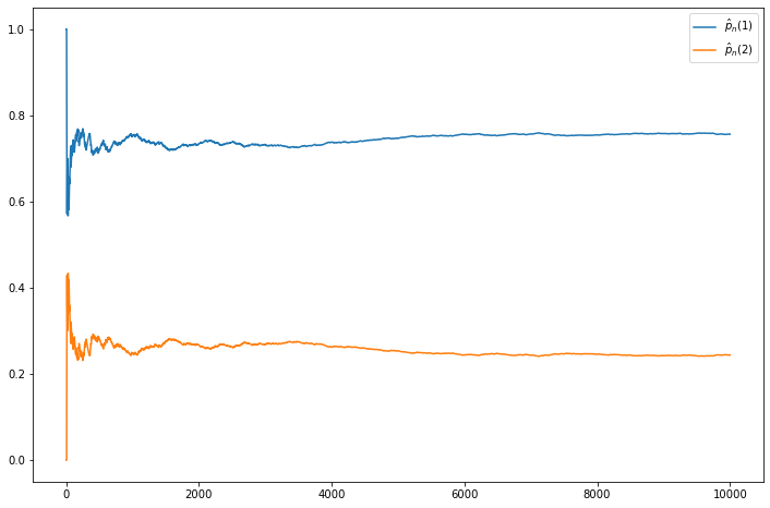
png
Note that the values do converge to \(\pi = (0.75, 0.25)\).
Exercise 24.6.5. An important Markov chain is the branching process which is used in biology, genetics, nuclear physics and many other fields. Suppose that an animal has \(Y\) children. Let \(p_k = \mathbb{P}(Y = k)\). Hence \(p_k \geq 0\) for all \(k\) and \(\sum_{k = 0}^\infty p_k = 1\). Assume each animal has the same lifespan and that they produce offspring according to the distribution \(p_k\). Let \(X_n\) be the number of animals in the \(n\)-th generation. Let \(Y_1^{(n)}, \dots, Y_{X_n}^{(n)}\) be the offspring produced in the \(n\)-th generation. Note that
\[ X_{n+1} = Y_1^{(n)} + \dots + Y_{X_n}^{(n)}\]
Let \(\mu = \mathbb{E}(Y)\) and \(\sigma^2 = \mathbb{V}(Y)\). Assume throughout this question that \(X_0 = 1\). Let \(M(n) = \mathbb{E}(X_n)\) and \(V(n) = \mathbb{V}(X_n)\).
(a) Show that \(M(n + 1) = \mu M(n)\) and that $V(n + 1) = ^2 M(n) + ^2 V(n) $.
(b) Show that \(M(n) = \mu^n\) and that \(V(n) = \sigma^2 \mu^{n-1} (1 + \mu + \dots + \mu^{n - 1})\).
(c) What happens to the variance if \(\mu > 1\)? What happens to the variance if \(\mu = 1\)? What happens to the variance if \(\mu < 1\)?
(d) The population goes extinct if \(X_n = 0\) for some \(n\). Let us thus define the extinction time \(N\) by
\[ N = \min \{ n : X_n = 0 \} \]
Let \(F(n) = \mathbb{P}(N \leq n)\) be the CDF of the random variable \(N\). Show that
\[ F(n) = \sum_{k=0}^\infty p_k \left( F(n - 1) \right)^k, \quad n = 1, 2, \dots \]
Hint: note that the event \(\{ N \leq n \}\) is the same event as \(\{ X_n = 0 \}\). Thus \(\mathbb{P}(N \leq n) = \mathbb{P}(X_n = 0)\). Let \(k\) be the number of offspring of the original event. The population becomes extinct at time \(n\) if and only if each of the \(k\) sub-populations generated from the \(k\) offspring goes extinct in \(n - 1\) generations.
(e) Suppose that \(p_0 = 1/4\), \(p_1 = 1/2\), \(p_2 = 1/4\). Use the formula from (d) to compute the CDF \(F(n)\).
Solution.
(a) We have:
\[ M(n + 1) = \mathbb{E}[X_{n + 1}] = \mathbb{E}\left[ \sum_{i = 1}^{X_n} Y_i^{(n)} \right] = \mathbb{E}\left[ \sum_{i = 1}^{X_n} \mathbb{E}[Y_i^{(n)}] \right] = \mathbb{E}\left[ \sum_{i = 1}^{X_n} \mu \right] = \mu \mathbb{E}[X_n] = \mu M(n)\]
We also have:
\[ \begin{align} V(n + 1) &= \mathbb{V}[X_{n + 1}] = \mathbb{E}[X_{n + 1}^2] - \mathbb{E}[X_{n + 1}]^2 \\ &= \mathbb{E}\left[\left( \sum_{i = 1}^{X_n} Y_i^{(n)} \right)^2\right] - \mu^2 M(n)^2 \\ &= \mathbb{E}\left[ \sum_{i = 1}^{X_n} \left( Y_i^{(n)} \right)^2 + \sum_{i = 1}^{X_n} \sum_{j = 1, j \neq i}^{X_n} Y_i^{(n)} Y_j^{(n)} \right] - \mu^2 M(n)^2 \\ &= \mathbb{E}\left[ \sum_{i = 1}^{X_n} \mathbb{E}\left[\left( Y_i^{(n)} \right)^2\right] + \sum_{i = 1}^{X_n} \sum_{j = 1, j \neq i}^{X_n} \mathbb{E}\left[ Y_i^{(n)} Y_j^{(n)} \right] \right] - \mu^2 M(n)^2 \\ &= \mathbb{E}\left[ \sum_{i = 1}^{X_n} \left( \mathbb{V}[Y_i^{(n)}] + \mathbb{E}\left[ Y_i^{(n)} \right]^2 \right) + \sum_{i = 1}^{X_n} \sum_{j = 1, j \neq i}^{X_n} \mathbb{E}\left[ Y_i^{(n)} \right] \mathbb{E} \left[ Y_j^{(n)} \right] \right] - \mu^2 M(n)^2 \\ &= \mathbb{E}\left[ \sum_{i = 1}^{X_n} \left( \sigma^2 + \mu^2 \right) + \sum_{i = 1}^{X_n} \sum_{j = 1, j \neq i}^{X_n} \mu^2 \right] - \mu^2 M(n)^2 \\ &= \mathbb{E} \left[ X_n (\sigma^2 + \mu^2) + X_n (X_n - 1) \mu^2 \right] - \mu^2 M(n)^2 \\ &= \mathbb{E} \left[ X_n \sigma^2 + X_n^2 \mu^2 \right] - \mu^2 M(n)^2 \\ &= \sigma^2 \mathbb{E} [ X_n ] + \mu^2 \mathbb{E} [ X_n^2 ] - \mu^2 M(n)^2 \\ &= \sigma^2 M(n) + \mu^2 (V(n) + M(n)^2) - \mu^2 M(n)^2 \\ &= \sigma^2 M(n) + \mu^2 V(n) \end{align} \]
(b)
Since the initial population is 1, \(M(0) = 1\); since \(M(n + 1) = \mu M(n)\), it follows by induction that \(M(n) = \mu^n\).
Now, we also have that the initial population is known, so \(V(0) = 0\). By induction,
\[ \begin{align} V(n + 1) &= \sigma^2 M(n) + \mu^2 V(n) \\ &= \sigma^2 \mu^n + \mu^2 \left( \sigma^2 \mu^{n - 1} \left( 1 + \mu + \dots + \mu^{n - 1}\right) \right) \\ &= \sigma^2 \mu^n \left(1 + \mu \left( 1 + \mu + \dots + \mu^{n - 1} \right) \right) \\ &= \sigma^2 \mu^n \left(1 + \mu + \dots + \mu^n \right) \end{align} \]
(c) If \(\mu \neq 1\), we can add up the geometric sum and write
\[ V(n) = \sigma^2 \mu^n \frac{1 - \mu^{n}}{1 - \mu}\]
- For \(\mu > 1\), \(V(n)\) grows exponentially.
- For \(\mu < 1\), \(V(n)\) converges to 0.
- For \(\mu = 1\), we have \(V(n) = n \sigma^2\), which grows linearly.
(d) Following the reasoning in the hint,
\[ \begin{align} F(n) &= \mathbb{P}(N \leq n) = \mathbb{P}(X_n = 0) \\ &= \sum_{k=0}^\infty \mathbb{P}(X_n = 0 | X_1 = k) \mathbb{P}(X_1 = k) \\ &= \sum_{k=0}^\infty \mathbb{P}(Y_i^{(n - 1)} = 0 \text{ for all } i | X_1 = k) \mathbb{P}(X_1 = k) \\ &= \sum_{k=0}^\infty \left( \prod_{i=1}^k \mathbb{P}(Y_i^{(n - 1)} = 0 | X_1 = k) \right) \mathbb{P}(X_1 = k) \\ &= \sum_{k=0}^\infty \left( \prod_{i=1}^k F(n-1) \right) p_k \\ &= \sum_{k=0}^\infty p_k \left( F(n - 1)\right)^k \end{align} \]
(e) The recurrence formula is:
\[ F(n + 1) = p_0 + p_1 F(n) + p_2 F(n)^2 = \frac{1}{4} + \frac{1}{2} F(n) + \frac{1}{4} F(n)^2 = \frac{1}{4} (F(n) + 1)^2\]
with initial value \(F(0) = 0\) (since we start with a non-extinct population).
import numpy as np

N = 1000
F = np.empty(N)

F[0] = 0
for n in range(1, N):
    F[n] = (F[n - 1] + 1)**2 / 4
import matplotlib.pyplot as plt
%matplotlib inline
plt.figure(figsize=(12, 8))
plt.plot(np.arange(1, N + 1), F)
plt.xlabel('N')
plt.ylabel('F(N)')
plt.xscale('log')
plt.show()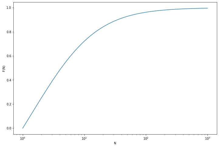
png
Exercise 24.6.6. Let
\[ P = \begin{bmatrix} 0.40 & 0.50 & 0.10 \\ 0.05 & 0.70 & 0.25 \\ 0.05 & 0.50 & 0.45 \end{bmatrix}\]
Find the stationary distribution \(\pi\).
Solution. The stationary distribution \(\pi\) satisfies \(\pi = \pi P\), so it is a (normalized) left eigenvector of \(P\), or a right eigenvector of \(P^T\).
import numpy as np
from numpy.linalg import eig

P = np.array([[0.4, 0.5, 0.1], [0.05, 0.7, 0.25], [0.05, 0.5, 0.45]])
w, v = eig(P.T)
pi = v[:, 0]
print(pi)[0.11041049 0.89708523 0.42784065]print(pi @ P)[0.11041049 0.89708523 0.42784065]Exercise 24.6.7. Show that if \(i\) is a recurrent state and \(i \leftrightarrow j\), then \(j\) is a recurrent state.
Solution.
Since \(i\) is recurrent, \(\sum_n p_{ii}(n) = \infty\). But
\[\sum_n p_{jj}(n) \geq \sum_{a, b, c} p_{ji}(a) p_{ii}(b) p_{ij}(c) \geq \sum_b p_{ji}(a') p_{ii}(b) p_{ij}(c')\]
for some \(a'\) such that \(p_{ji}(a') > 0\) (which exists because \(j \rightarrow i\)) and some \(c'\) such that \(p_{ij}(c') > 0\) (which exists because \(i \rightarrow j\)). Then this sum is lower bounded by
\[\frac{1}{p_{ji}(a') p_{ij}(c')} \sum_b p_{ii}(b)\]
which diverges because \(\sum_n p_{ii}(n) = \infty\), so \(j\) must be a recurrent state.
Exercise 24.6.8. Let
\[ P = \begin{bmatrix} 1/3 & 0 & 1/3 & 0 & 0 & 1/3 \\ 1/2 & 1/4 & 1/4 & 0 & 0 & 0 \\ 0 & 0 & 0 & 0 & 1 & 0 \\ 1/4 & 1/4 & 1/4 & 0 & 0 & 1/4 \\ 0 & 0 & 1 & 0 & 0 & 0 \\ 0 & 0 & 0 & 0 & 0 & 1 \end{bmatrix}\]
Which states are transient? Which states are recurrent?
Solution.
from graphviz import Digraph

d = Digraph()

d.edge('1', '1', label='1/3')
d.edge('1', '3', label='1/3')
d.edge('1', '6', label='1/3')

d.edge('2', '1', label='1/2')
d.edge('2', '2', label='1/4')
d.edge('2', '3', label='1/4')

d.edge('3', '5', label='1')

d.edge('4', '1', label='1/4')
d.edge('4', '2', label='1/4')
d.edge('4', '3', label='1/4')
d.edge('4', '6', label='1/4')

d.edge('5', '3', label='1')

d.edge('6', '6', label='1')

d
svg
States 3, 5, 6 are recurrent:
- A chain starting on state 6 will forever stay in state 6.
- A chain starting on states 3 or 5 will bounce between states 3 and 5 forever.
Other states are not recurrent, as they may eventually fall into state 6 and never reach other state after.
Exercise 24.6.9. Let
\[ P = \begin{bmatrix} 0 & 1 \\ 1 & 0 \end{bmatrix}\]
Show that \(\pi = (1/2, 1/2)\) is a stationary distribution. Does this chain converge? Why / why not?
Solution. The distribution is stationary if and only if \(\pi = \pi P\), and
\[ \pi P = \begin{bmatrix} 1/2 & 1/2 \end{bmatrix} \begin{bmatrix} 0 & 1 \\ 1 & 0 \end{bmatrix} = \begin{bmatrix} 1/2 & 1/2 \end{bmatrix} = \pi \]
This chain does not converge: it will always oscillate between states 1 and 2 with probability 1.
Exercise 24.6.10. Let \(0 < p < 1\) and \(q = 1 - p\). Let
\[ P = \begin{bmatrix} q & p & 0 & 0 & 0 \\ q & 0 & p & 0 & 0 \\ q & 0 & 0 & p & 0 \\ q & 0 & 0 & 0 & p \\ 1 & 0 & 0 & 0 & 0 \end{bmatrix} \]
Find the limiting distribution of the chain.
Solution.
Solving \(\pi P = \pi\), we get:
\[ \pi = \begin{bmatrix} \frac{1 - p}{p^4(1 - p^5)} & \frac{1 - p}{p^3(1 - p^5)} & \frac{1 - p}{p^2(1 - p^5)} & \frac{1 - p}{p(1 - p^5)} & \frac{1 - p}{1 - p^5} \end{bmatrix} \]
We can verify this is the limiting distribution:
\[ \begin{align} \pi P &= \begin{bmatrix} \frac{1 - p}{p^4(1 - p^5)} & \frac{1 - p}{p^3(1 - p^5)} & \frac{1 - p}{p^2(1 - p^5)} & \frac{1 - p}{p(1 - p^5)} & \frac{1 - p}{1 - p^5} \end{bmatrix} \begin{bmatrix} 1 - p & p & 0 & 0 & 0 \\ 1 - p & 0 & p & 0 & 0 \\ 1 - p & 0 & 0 & p & 0 \\ 1 - p & 0 & 0 & 0 & p \\ 1 & 0 & 0 & 0 & 0 \end{bmatrix} \\ &= \begin{bmatrix} \frac{(1 - p)^2}{p^4(1 - p^5)} + \frac{(1 - p)^2}{p^3(1 - p^5)} + \frac{(1 - p)^2}{p^2(1 - p^5)} + \frac{(1 - p)^2}{p(1 - p^5)} + \frac{1 - p}{1 - p^5} & \frac{1 - p}{p^3(1 - p^5)} & \frac{1 - p}{p^2(1 - p^5)} & \frac{1 - p}{p(1 - p^5)} & \frac{1 - p}{1 - p^5} \end{bmatrix} \\ &= \begin{bmatrix} \frac{(1 - p)^2(1 + p + p^2 + p^3) + p^4(1 - p)}{p^4(1 - p^5)} & \frac{1 - p}{p^3(1 - p^5)} & \frac{1 - p}{p^2(1 - p^5)} & \frac{1 - p}{p(1 - p^5)} & \frac{1 - p}{1 - p^5} \end{bmatrix} \\ &= \begin{bmatrix} \frac{1 - p}{p^4(1 - p^5)} & \frac{1 - p}{p^3(1 - p^5)} & \frac{1 - p}{p^2(1 - p^5)} & \frac{1 - p}{p(1 - p^5)} & \frac{1 - p}{1 - p^5} \end{bmatrix} \\ &= \pi \end{align} \]
Exercise 24.6.11. Let \(X(t)\) be an inhomogeneous Poisson process with intensity function \(\lambda(t) > 0\). Let \(\Lambda(t) = \int_0^t \lambda(u) du\). Define \(Y(s) = X(t)\) where \(s = \Lambda(t)\). Show that \(Y(s)\) is a homogeneous Poisson process with intensity \(\lambda = 1\).
Solution.
We have: \(Y(s) = X(\Lambda^{-1}(s))\) and \(X(t) \sim \text{Poisson}(\Lambda(t))\), so
\[Y(s) \sim \text{Poisson}(\Lambda(\Lambda^{-1}(s)) = \text{Poisson}(s) = \text{Poisson}(\lambda_Y \cdot s)\]
which is the desired result with \(\lambda_Y = 1\).
Exercise 24.6.12. Let \(X(t)\) be a Poisson process with intensity \(\lambda\). Find the conditional distribution of \(X(t)\) given that \(X(t + s) = n\).
Solution. The random variables \(X(t) - X(0) = X(t)\) and \(Y(s) = X(t + s) - X(t)\) are independent, as they are both count increments, with \(X(t) \sim \text{Poisson}(\lambda t)\) and \(Y(s) \sim \text{Poisson}(\lambda s)\). Then:
\[ \begin{align} \mathbb{P}\left(X(t) = x | X(t + s) = n\right) &= \mathbb{P}\left(X(t) = x | X(t) + Y(s) = n\right) \\ &= \frac{\mathbb{P}\left(X(t) = x, X(t) + Y(s) = n\right)}{\mathbb{P}\left(X(t) + Y(s) = n\right)} \\ &= \frac{\mathbb{P}\left(X(t) = x, Y(s) = n - x\right)}{\sum_{0 \leq j \leq n} \mathbb{P}\left(X(t) = j, Y(s) = n - j\right)} \\ &= \frac{\mathbb{P}\left(X(t) = x\right) \mathbb{P}\left(Y(s) = n - x\right)}{\sum_{j=0}^n \mathbb{P}\left(X(t) = j\right) \mathbb{P}\left( Y(s) = n - j\right)} \\ &= \frac{f(x)}{\sum_{j=0}^n f(j) } \end{align} \]
where \(f(x) = \mathbb{P}\left(X(t) = x\right) \mathbb{P}\left( Y(s) = n - x\right)\). But we have:
\[ f(x) = \frac{(\lambda t)^x e^{-\lambda t}}{x!}\frac{(\lambda s)^{n - x} e^{-\lambda s}}{(n - x)!} = \frac{\lambda^n e^{-\lambda (t + s)}}{n!} \binom{n}{x} t^x s^{n - x} \]
Replacing on the expression above and cancelling the factors that do not depend on \(x\), we get
\[ \mathbb{P}\left(X(t) = x | X(t + s) = n\right) = \frac{f(x)}{\sum_{j=0}^n f(j) } = \frac{\binom{n}{x} t^x s^{n - x}}{\sum_{j=0}^n \binom{n}{j} t^j s^{n - j}} = \frac{\binom{n}{x} t^x s^{n - x}}{(t + s)^n} = \binom{n}{x} \left( \frac{t}{t + s} \right)^x \left( \frac{s}{t + s}\right)^{n - x}\]
using the binomial expansion \((t + s)^n = \sum_{j=0}^n \binom{n}{j} t^j s^{n - j}\). Therefore, the conditional distribution follows a Binomial distribution,
\[ X(t)=x | X(t + s)=n \sim \text{Binomial}\left(n, \frac{t}{t + s} \right)\]
Exercise 24.6.13. Let \(X\) be a Poisson process with intensity \(\lambda\). Find the probability that \(X(t)\) is odd, i.e. \(\mathbb{P}(X(t) = 1, 3, 5, \dots)\).
Solution. Expanding using the probability mass function,
\[\begin{align} \mathbb{P}(X(t) \text{ is odd}) &= \sum_{k=0}^\infty \frac{(\lambda t)^{2k + 1} e^{-\lambda t}}{(2k + 1)!} \\ &=e^{-\lambda t}\frac{1}{2}\left(\sum_{0}^{+\infty}\frac{(\lambda t)^n}{n!}-\sum_{0}^{+\infty}\frac{(-\lambda t)^n}{n!}\right)\\ &=e^{-\lambda t}\frac{1}{2}\left(e^{(\lambda t)}-e^{-(\lambda t)}\right)\\ &=e^{-\lambda t} \text{sinh} (\lambda t) \\ &= \frac{1}{2}\left( 1 - e^{-2 \lambda t}\right) \end{align}\]
Exercise 24.6.14. Suppose that people logging in to the University computer system is described by a Poisson process \(X(t)\) with intensity \(\lambda\). Assume that a person stays logged in for some random time with CDF \(G\). Assume these times are all independent. Let \(Y(t)\) be the number of people on the system at time \(t\). Find the distribution of \(Y(t)\).
Solution.
The number of people arriving at time period \(j\) is \(A(j) \equiv X(j) - X(j-1)\), where \(X(0) = 0\). Let \(W_i^{(j)}\) be the amount of time spent by the \(i\)-th person that arrived at time period \(j\). Then, the total number of people at time \(t\) is:
\[ Y(t) = \sum_{j=1}^t \sum_{i=1}^{A(j)} I\left(W_i^{(j)} \geq t - j\right) \]
where \(I(x) = 1\) if \(x\) is true and \(0\) otherwise, and the terms count only the people who are still logged in after an extra time \(t - j\) elapsed.
Each value \(I\left(W_i^{(j)} \geq x\right)\) follows a distribution given by \(1 - G(x)\), measuring the probability of a person staying longer than time \(x\), and they are all independent.
We can write the sum above as:
\[ Y(t) = \sum_{j=1}^t B(j), \quad B(j) =\sum_{i = 1}^{A(j)} I\left(W_i^{(j)} \geq t - j\right) \]
Note that this implies that \(B(j) | A(j) = n\) follows a binomial distribution with parameters \(n\) and \(\mathbb{P}\left(W_i^{(j)} \geq t - j \right) = 1 - G(t - j)\).
Since \(A(j) \sim \text{Poisson}(\lambda)\) and \(B(j) | A(j) = n \sim \text{Binomial}(n, 1 - G(t - j))\), the marginal distribution of \(B(j)\) is \(B(j) \sim \text{Poisson}\left(\lambda (1 - G(t - j))\right)\). Therefore, \(Y\) being the sum of independent Poisson variables \(B(j)\), we get that \(Y\) is a Poisson process with inhomogeneous rate \(\lambda_Y(t)\),
\[ Y(t) \sim \text{Poisson}\left( \lambda_Y(t) \right), \quad \lambda_Y(t) = \lambda \left[ \sum_{j=1}^t(1 - G(t - j)) \right]\]
Exercise 24.6.15. Let \(X(t)\) be a Poisson process with intensity \(\lambda\). Let \(W_1, W_2, \dots\) be the waiting times. Let \(f\) be an arbitrary function. Show that
\[ \mathbb{E} \left[ \sum_{i=1}^{X(t)} f(W_i) \right] = \lambda \int_0^t f(w) dw \]
Solution.
When conditioning on \(X(t) = n\), the waiting times are uniformly distributed on the interval \([0, t]\), so \(\sum_{i=1}^n f(W_i)\) has the same distribution as \(\sum_{i=1}^n f\left(U_i^{(n)}\right)\), for \(U_i^{(n)} \sim \text{Uniform}(0, t)\). Then the expectation of \(f\left(U_i^{(n)}\right)\) is
\[\mathbb{E}\left[ f\left(U_i^{(n)}\right) \right] = \int_0^t f(w) f_{U_i^{(n)}}(w) dw = \frac{1}{t} \int_0^t f(w) dw\]
Then, we have:
\[ \begin{align} \mathbb{E}\left[ \sum_{i=1}^{X(t)} f(W_i) \right] &= \sum_{n = 0}^\infty \mathbb{E}\left[ \sum_{i=1}^{X(t)} f(W_i) \; \Bigg| \; X(t) = n\right] \mathbb{P} \left[ X(t) = n \right] \\ &= \sum_{n = 0}^\infty \mathbb{E}\left[ \sum_{i=1}^n f\left(U_i^{(n)}\right) \right] \mathbb{P} \left[ X(t) = n \right] \\ &= \sum_{n = 0}^\infty \frac{n}{t} \left( \int_0^t f(w) dw \right) \mathbb{P} \left[ X(t) = n \right] \\ &= \frac{1}{t} \left( \int_0^t f(w) dw \right) \sum_{n=0}^\infty n \; \mathbb{P} \left[ X(t) = n \right] \\ &= \frac{1}{t} \left( \int_0^t f(w) dw \right) \mathbb{E} \left[ X(t) \right] \\ &= \frac{1}{t} \left( \int_0^t f(w) dw \right) \lambda t \\ &= \lambda \int_0^t f(w) dw \end{align} \]
Exercise 24.6.16. A two dimensional Poisson process is a process of random points in the plane such that (i) for any set \(A\), the number of points falling in \(A\) is Poisson with mean \(\lambda \mu(A)\) where \(\mu(A)\) is the area of \(A\), (ii) the number of points in nonoverlapping regions is independent. Consider an arbitrary point \(x_0\) in the plane. Let \(X\) denote the distance from \(x_0\) to the nearest point. Show that
\[ \mathbb{P}(X > t) = e^{-\lambda \pi t^2} \]
and
\[ \mathbb{E}(X) = \frac{1}{2 \sqrt{\lambda}} \]
Solution. The distance \(X\) from \(x_0\) to the nearest point is at least \(t\) if and only if no points lie within a circle of radius \(t\) centered in \(x_0\). This circle \(C\) has area \(\mu(C) = \pi t^2\), and so
\[ \mathbb{P}(X > t) = \mathbb{P}(\# \{\text{points in C} \} = 0) = f_C(0) = \frac{\lambda_C^0 e^{-\lambda_C}}{0!} = e^{-\lambda_C} = e^{-\lambda \pi t^2} \]
Given that \(X\) has a CDF of \(F_X(x) = 1 - e^{-\lambda \pi x^2}\) for \(x \geq 0\), its PDF is \(f_X(x) = 2 \lambda \pi x e^{-\lambda \pi x^2}\), and its mean is
\[\begin{align} \mathbb{E}(X) &= \int_0^\infty x f_X(x) \; dx \\ &= \int_0^\infty 2 \lambda \pi x^2 e^{- \lambda \pi x^2} \; dx \\ &=-\int_0^\infty xe^{- \lambda \pi x^2}d(- \lambda \pi x^2)\\ &=-xe^{- \lambda \pi x^2}\big|_{0}^{\infty}+\int_0^\infty e^{- \lambda \pi x^2}dx\\ &=\int_0^\infty e^{- \lambda \pi x^2}dx\\ &=\frac{1}{\sqrt{\lambda \pi}}\int_0^\infty e^{- (\sqrt{\lambda \pi} x)^2}d(\sqrt{\lambda \pi} x)\\ &= \frac{1}{\sqrt{\lambda \pi}}\sqrt{\pi}/2\\ &= \frac{1}{2 \sqrt{\lambda}} \end{align}\]
Since \[\int_{-\infty}^{+\infty}e^{-x^2}dx=\sqrt{\pi}\] Let \[\int_{-\infty}^{+\infty}e^{-x^2}dx=I\] \[\begin{align} I^2&=\left(\int_{-\infty}^{+\infty}e^{-x^2}dx\right)×\left(\int_{-\infty}^{+\infty}e^{-y^2}dy\right)\\ &=\int_{-\infty}^{+\infty}\left(\int_{-\infty}^{+\infty}e^{−(x^2+y^2)}dx\right)dy\\ &=\int\int e^{−(r^2)}rd\theta dr\\ &=\int_0^{2\pi} \left(\int_{0}^{+\infty}re^{−r^2}dr\right)d\theta\\ &=2\pi\int_{0}^{+\infty}re^{−r^2}dr\\ &=\pi\int_{0}^{+\infty}2re^{−r^2}dr\\ &=\pi\int_{0}^{+\infty}e^{−r^2}d(r^2)\\ &=\pi \end{align}\]
The polar form: \[x^2+y^2=r^2, dxdy=dA=rd\theta dr\]