22. Smoothing Using Orthogonal Functions
In this Chapter we study a different approach to nonparametric curve estimation based on orthogonal functions. We begin with a brief introduction to the theory of orthogonal functions. Then we turn to density estimation and regression.
22.1 Orthogonal Functions and \(L_2\) Spaces
Let \(v = (v_1, v_2, v_3)\) denote a three dimensional vector. Let \(\mathcal{V}\) denote the set of all such vectors.
- If \(a\) is a scalar and \(v\) is a vector, we define \(av = (av_1, av_2, av_3)\).
- The sum of vectors \(v\) and \(w\) is defined as \(v + w = (v_1 + w_1, v_2 + w_2, v_3 + w_3)\).
- The inner product between vectors \(v\) and \(w\) is defined by \(\langle v, w \rangle = \sum_i v_i w_i\).
- The norm (or length) of a vector is defined by
\[ \Vert v \Vert = \sqrt{\langle v, v \rangle} = \sqrt{\sum_i v_i^2 }\]
- Two vectors are orthogonal (or perpendicular) if \(\langle v, w \rangle = 0\).
- A set of vectors are orthogonal if each pair in the set is orthogonal.
- A vector is normal if \(\Vert v \Vert = 1\).
Let \(\phi_1 = (1, 0, 0)\), \(\phi_2 = (0, 1, 0)\), \(\phi_3 = (0, 0, 1)\). These vectors are said to be an orthonormal basis for \(\mathcal{V}\) since they have the following properties:
- they are orthogonal
- they are normal
- they form a basis for \(\mathcal{V}\), that is, if \(v \in \mathcal{V}\) then \(v\) can be written as a linear combination of \(\phi_i\),
\[v = \sum_i \beta_i \phi_i \quad \text{where } \beta_i = \langle \phi_i, v \rangle\]
There are other orthonormal basis for \(\mathcal{V}\), for example
\[ \psi_1 = \left( \frac{1}{\sqrt{3}}, \frac{1}{\sqrt{3}} , \frac{1}{\sqrt{3}} \right), \quad \psi_2 = \left( \frac{1}{\sqrt{2}}, -\frac{1}{\sqrt{2}} , 0 \right), \quad \psi_3 = \left( \frac{1}{\sqrt{6}}, \frac{1}{\sqrt{6}} , -\frac{2}{\sqrt{6}} \right) \]
Now we make the leap from vectors to functions. Basically, we just replace vectors with functions and sums with integrals.
Let \(L_2(a, b)\) denote all functions defined on the interval \([a, b]\) such that \(\int_a^b f(x)^2 dx < \infty\):
\[ L_2(a, b) = \left\{ f: [a, b] \rightarrow \mathbb{R} , \int_a^b f(x)^2 < \infty \right\} \]
We sometimes write \(L_2\) instead of \(L_2(a, b)\).
- The inner product between two functions \(f, g \in L_2\) is \(\langle f, g \rangle = \int f(x) g(x) dx\).
- The norm of \(f\) is
\[ \Vert f \Vert = \sqrt{\int f(x)^2 dx} \]
- Two functions are orthogonal if \(\langle f, g \rangle = 0\).
- A function is normal if \(\Vert f \Vert = 1\).
- A sequence of functions \(\phi_1, \phi_2, \phi_3, \dots\) is orthonormal if \(|| \phi_i || = 1\) for each \(i\) and \(\langle \phi_i, \phi_j \rangle = 0\) for \(i \neq j\).
- An orthonormal sequence is complete if the only function that is orthogonal to each \(\phi_i\) is the zero function. In that case, the functions \(\phi_1, \phi_2, \phi_3, \dots\) form a basis, meaning that if \(f \in L_2\) then \(f\) can be written as
\[ f(x) = \sum_{j=1}^\infty \beta_j \phi_j(x) \quad \text{where } \beta_j = \int_a^b f(x) \phi_j(x) dx \]
Parseval’s relation says that
\[ \Vert f \Vert^2 \equiv \int f^2(x) dx = \sum_{j=1}^\infty \beta_j^2 \equiv \Vert \beta \Vert^2\]
The cosine basis is defined as follows: Let \(\phi_1(x) = 1\) and for \(j \geq 2\) define
\[\phi_j(x) = \sqrt{2} \cos \left( (j - 1) \pi x\right)\]
The first ten functions are plotted below.
import numpy as np

def cosine_basis(j):
    assert j >= 1

    def f(x):
        if j == 1:
            return np.ones_like(x)
        return np.sqrt(2) * np.cos((j - 1) * np.pi * x)

    return f
import matplotlib.pyplot as plt
%matplotlib inline
step = 1e-3
xx = np.arange(0, 1 + step, step=step)
plt.figure(figsize=(12, 12))
for i in range(1, 11):
# Set up the plot
ax = plt.subplot(5, 2, i)
ax.plot(xx, cosine_basis(i)(xx))
ax.set_title('j = %i' % i)
plt.tight_layout()
plt.show()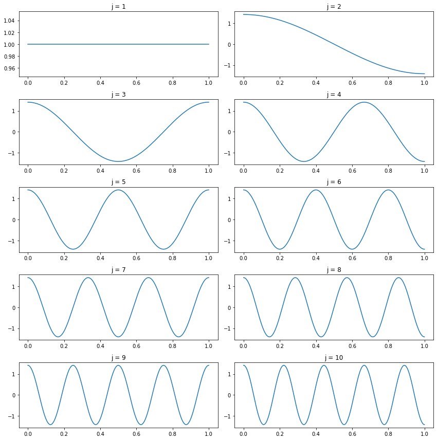
png
The Legendre polynomials on \([-1, 1]\) are defined by
\[ P_j(x) = \frac{1}{2^j j!} \frac{d^j}{dx^j} (x^2 - 1)^j, \quad j = 0, 1, 2, \dots \]
It can be shown that these functions are complete and orthogonal, and that
\[ \int_{-1}^1 P_j^2(x) dx = \frac{2}{2j + 1}\]
It follows that the functions
\[ \phi_j(x) = \sqrt{\frac{2j + 1}{2}}P_j(x), \quad j = 0, 1, 2, \dots \]
form an orthonormal basis for \(L_2[-1, 1]\). The first few Legendre polynomials are
\[ \begin{align} P_0(x) &= 1 \\ P_1(x) &= x \\ P_2(x) &= \frac{1}{2}\left( 3x^2 - 1 \right) \\ P_3(x) &= \frac{1}{2}\left( 5x^3 - 3x \right) \end{align} \]
These polynomials may be constructed explicitly using the following recursive relation:
\[ P_{j+1}(x) = \frac{(2j + 1) x P_j(x) - j P_{j - 1}(x)}{j + 1} \]
import sympy
from sympy.abc import x
from functools import lru_cache

@lru_cache(maxsize=None)
def legendre_polynomial(j):
    if j == 0:
        return 1
    if j == 1:
        return x

    return sympy.expand(((2*j - 1) * x * legendre_polynomial(j - 1) - (j - 1) * legendre_polynomial(j - 2)) / j)

def legendre_basis(j):
    if j == 0:
        return lambda x: np.sqrt(1/2) * np.ones_like(x)

    pj = legendre_polynomial(j)
    return sympy.lambdify(x, sympy.sqrt((2*j + 1) / 2) * pj, "numpy")
import matplotlib.pyplot as plt
%matplotlib inline
step = 1e-3
xx = np.arange(-1, 1 + step, step=step)
plt.figure(figsize=(12, 12))
for i in range(0, 10):
# Set up the plot
ax = plt.subplot(5, 2, i + 1)
ax.plot(xx, legendre_basis(i)(xx))
ax.set_title('j = %i' % i)
plt.tight_layout()
plt.show()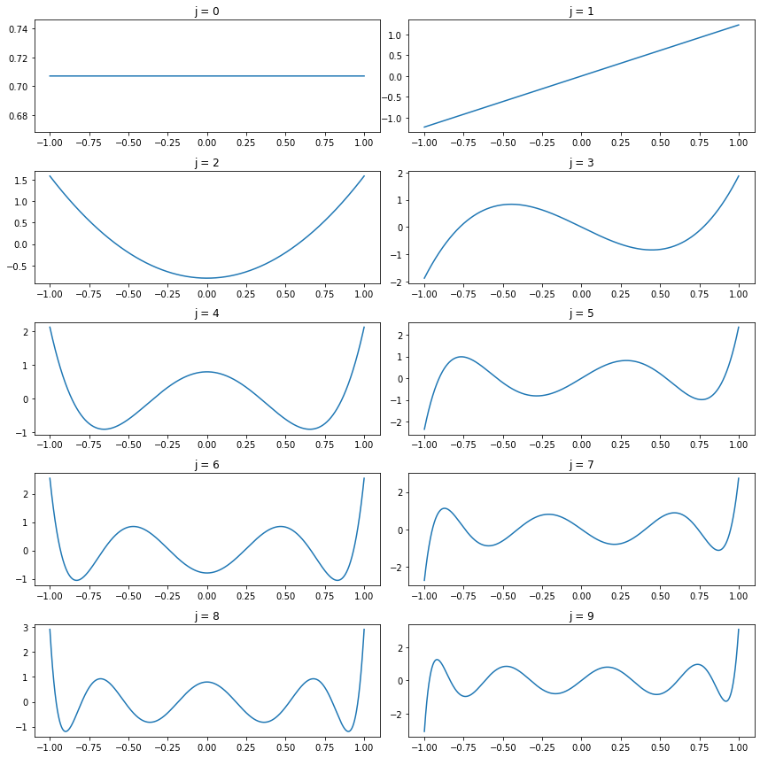
png
The coefficients \(\beta_1, \beta_2, \dots\) are related to the smoothness of the function \(f\). To see why note that, if \(f\) is smooth, then its derivative will be finite. Thus we expect that, for some \(k\), \(\int_0^1 (f^{(k)}(x))^2 dx < \infty\), where \(f^{(k)}\) is the \(k\)-th derivative of \(f\).
Now consider the cosine basis and let \[f(x) = \sum_{j=1}^\infty \beta_j \phi_j(x)=\sum_{j=1}^\infty \beta_j\sqrt{2} \cos \left( (j - 1) \pi x\right)\] Then,
\[ \int_0^1 (f^{(k)}(x))^2 dx \le 2 \sum_{j=1}^\infty \beta_j^2 ( \pi (j - 1) ) ^{2k} \]
The only way the sum can be finite is if the \(\beta_j\)’s get small when \(j\) gets large. To summarize:
If the function \(f\) is smooth then the coefficients \(\beta_j\) will be small when \(j\) is large.
For the rest of this chapter, we will assume we are using the cosine basis unless otherwise specified.
22.2 Density Estimation
Let \(X_1, \dots, X_n\) be IID observations from a distribution on \([0, 1]\) with density \(f\). Assuming \(f \in L_2\) we can write
\[ f(x) = \sum_{j=1}^\infty \beta_j \phi_j(x) \]
where \(\phi_i\)s form an orthonormal basis. Define
\[ \hat{\beta}_j = \frac{1}{n} \sum_{i=1}^n \phi_j(X_i)\]
Theorem 22.4. The mean and variance of the \(\hat{\beta}_j\) are
\[ \mathbb{E}(\hat{\beta}_j) = \beta_j \quad \text{and} \quad \mathbb{V}(\hat{\beta}_j) = \frac{\sigma_j^2}{n} \]
where
\[ \sigma_j^2 = \mathbb{V}(\phi_j(X_i)) = \int \left( \phi_j(x) - \beta_j\right)^2f(x) dx\]
Proof. We have
\[ \mathbb{E}(\hat{\beta}_j) = \frac{1}{n} \sum_{i=1}^n \mathbb{E}(\phi_j(X_i)) = \mathbb{E}(\phi_j(X_1)) = \int \phi_j(x) f(x) dx = \beta_j\]
The calculation for variance is similar:
\[ \mathbb{V}(\hat{\beta}_j) = \frac{1}{n^2} \sum_{i=1}^n \mathbb{V}(\phi_j(X_i)) = \frac{1}{n} \mathbb{V}(\phi_j(X_1)) = \frac{1}{n} \int \left( \phi_j(x) - \beta_j\right)^2f(x) dx \]
Hence, \(\hat{\beta}_j\) is an unbiased estimate of \(\beta_j\). It is tempting to estimate \(f\) by \(\sum_{i=1}^\infty \hat{\beta}_j \phi_j(x)\) but it turns out to have a very high variance. Instead, consider the estimator
\[ \hat{f}(x) = \sum_{i=1}^J \hat{\beta}_j \phi_j(x) \]
The number of terms \(J\) is a smoothing parameter. Increasing \(J\) will decrease bias while increasing variance. For technical reasons, we restrict \(J\) to lie in the range \(1 \leq J \leq p\) where \(p = p(n) = \sqrt{n}\). To emphasize the dependence of the risk function on \(J\), we write the risk function as \(R(J)\).
Theorem 22.5. The risk of \(\hat{f}\) is given by
\[ R(J) = \sum_{j=1}^J \frac{\sigma_j^2}{J} + \sum_{j=J+1}^\infty \beta_j^2 \]
In kernel estimation, we used cross-validation to estimate the risk. In the orthogonal function approach, we instead use the risk estimator
\[ \hat{R}(J) = \sum_{j=1}^J \frac{\hat{\sigma}_j^2}{n} + \sum_{j=J+1}^p \left( \hat{\beta}_j^2 - \frac{\hat{\sigma}_j^2}{n} \right)_{+}\]
where \(a_{+} = \max \{ a, 0 \}\) and
\[ \hat{\sigma}_j^2 = \frac{1}{n - 1} \sum_{i=1}^n \left( \phi_j(X_i) - \hat{\beta}_j\right)^2 \]
To motivate this estimator, note that \(\hat{\sigma}_j^2\) is an unbiased estimator of \(\sigma^2\) and \(\hat{\beta}_j^2 - \hat{\sigma}_j^2\) is an unbiased estimator of \(\beta_j^2\). We take the positive part of the later term since we know \(\beta_j^2\) cannot be negative. We now choose \(1 \leq \hat{J} \leq p\) to minimize the risk estimator \(\hat{R}(\hat f, f)\).
Summary of Orthogonal Function Density Estimation
- Let
\[ \hat{\beta}_j = \frac{1}{n} \sum_{i=1}^n \phi_j(X_i) \]
- Choose \(\hat{J}\) to minimize \(\hat{R}(J)\) over \(1 \leq J \leq p = \sqrt{n}\) where
\[ \hat{R}(J) = \sum_{j=1}^J \frac{\hat{\sigma}_j^2}{n} + \sum_{j=J+1}^p \left( \hat{\beta}_j^2 - \frac{\hat{\sigma}_j^2}{n} \right)_{+}\]
and
\[ \hat{\sigma}_j^2 = \frac{1}{n - 1} \sum_{i=1}^n \left( \phi_j(X_i) - \hat{\beta}_j\right)^2 \]
- Let
\[ \hat{f}(x) = \sum_{j=1}^\hat{J} \hat{\beta}_j \phi_j(x) \]
The estimator \(\hat{f}_n\) can be negative. If we are interested in estimating the shape of \(f\), this is not a problem. However, if we need the estimate to be a probability density function, we can truncate the estimate and then normalize it:
\[\hat{f}^*(x) = \frac{\max \{ \hat{f}_n(x), 0 \}}{\int_0^1 \max \{ \hat{f}_n(u), 0 \} du}\]
Now, let us construct a confidence band for \(f\). Suppose we estimate \(f\) using \(J\) orthogonal functions. We are essentially estimating \(\tilde{f}(x) = \sum_{j=1}^J \beta_j \phi_j(x)\) instead of the true density \(f(x) = \sum_{j=1}^\infty \beta_j \phi_j(x)\). Thus the confidence band should be regarded as a band for \(\tilde{f}(x)\).
Theorem 22.6. An approximate \(1 - \alpha\) confidence band for \(\tilde{f}\) is \((\ell(x), u(x))\) where
\[ \ell(x) = \hat{f}_n(x) - c \quad \text{and} \quad u(x) = \hat{f}_n(x) + x \]
where
\[ c = \frac{JK^2}{\sqrt{n}} \sqrt{1 + \frac{\sqrt{2} z_{\alpha}}{\sqrt{J}}} \]
and
\[ K = \max_{1 \leq j \leq J} \max_x | \phi_j(x) | \]
For the cosine basis, \(K = \sqrt{2}\).
22.3 Regression
Consider the regression model
\[ Y_i = r(x_i) + \epsilon_i, \quad i = 1, \dots, n\]
where \(\epsilon_i\) are independent with mean 0 and variance \(\sigma^2\). We will initially focus on the special case where \(x_i = i / n\). We assume that \(r \in L_2[0, 1]\) and hence we can write
\[ r(x) = \sum_{j=1}^\infty \beta_j \phi_j(x) \quad \text{where } \beta_j = \int_0^1 r(x) \phi_j(x) dx \]
where \(\phi_1, \phi_2, \dots\) is an orthonormal basis for \([0, 1]\).
Define
\[ \hat{\beta}_j = \frac{1}{n} \sum_{i=1}^n Y_i \phi_j(x), \quad j = 1, 2, \dots\]
Since \(\hat{\beta}_j\) is an average, the central limit theorem tells us that \(\hat{\beta}_j\) will be approximately normally distributed.
Theorem 22.8.
\[ \hat{\beta}_j \approx N \left( \beta_j, \frac{\sigma^2}{n} \right) \]
Proof. The mean of \(\hat{\beta}_j\) is
\[ \mathbb{E}(\hat{\beta}_j) = \frac{1}{n} \sum_{i=1}^n \mathbb{E}(Y_i) \phi_j(x_i) = \frac{1}{n} \sum_{i=1}^n r(x_i) \phi_j(x_i) \approx \int r(x) \phi_j(x) dx = \beta_j\]
where the approximate equality follows from the definition of a Riemann integral: \(\sum_i h(x_i) / n \rightarrow \int_0^1 h(x) dx\).
The variance is
\[ \mathbb{V}(\hat{\beta}_j) = \frac{1}{n^2} \sum_{i=1}^n \mathbb{V}(Y_i) \phi_j(x_i) = \frac{\sigma^2}{n} \left( \frac{1}{n} \sum_{i=1}^n \phi_j^2(x_i) \right) \approx \frac{\sigma^2}{n} \left( \int \phi_j^2(x) dx \right) = \frac{\sigma^2}{n}\]
since \(\phi_j\) has norm 1.
As we did for density estimation, we will estimate \(r\) by
\[ \hat{r}(x) = \sum_{j=1}^J \hat{\beta}_j \phi_j(x) \]
Let
\[ R(J) = \mathbb{E} \int (r(x) - \hat{r}(x))^2 dx \]
be the risk of the estimator.
Theorem 22.9. The risk \(R(J)\) of the estimator $ (x) = _{j=1}^J _j _j(x) $ is
\[ R(J) = \frac{J \sigma^2}{n} + \sum_{j=J+1}^\infty \beta_j^2 \]
To motivate the estimator \(\sigma^2 = \mathbb{V}(\epsilon_i)\) we use
\[ \hat{\sigma}^2 = \frac{n}{k} \sum_{i=n - k + 1}^n \hat{\beta}_j^2 \]
where \(k = n / 4\). To motivate this estimator, recall that if \(f\) is smooth then \(\beta_j \approx 0\) for large \(j\). So, for \(j \geq k\), \(\hat{\beta}_j \approx N(0, \sigma^2 / n)\). So \(\hat{\beta}_j \approx \sigma Z_j / \sqrt{n}\) for \(j \geq k\), where \(Z_j \sim N(0, 1)\). Therefore,
\[ \hat{\sigma}^2 = \frac{n}{k} \sum_{i=n-k+1}^k \hat{\beta}_j^2 \approx \frac{n}{k} \sum_{i=n-k+1}^k \left( \frac{\sigma}{\sqrt{n}} Z_j \right)^2 = \frac{\sigma^2}{k} \sum_{i=n-k+1}^k Z_j^2 = \frac{\sigma^2}{k} \chi_k^2\]
since a sum of \(k\) squares of independent standard normals has a \(\chi_k^2\) distribution. Now \(\mathbb{E}(\chi_k^2) = k\), leading to \(\mathbb{E}(\hat{\sigma}^2) \approx \sigma^2\). Also, \(\mathbb{V}(\chi_k^2) = 2k\) and so \(\mathbb{V}(\hat{\sigma}^2) \approx (\sigma^4 / k^2) 2k = 2\sigma^4 / k \rightarrow 0\) as \(n \rightarrow \infty\). Thus we expect \(\hat{\sigma}^2\) to be a consistent estimator of \(\sigma^2\).
There is nothing special about the choice of \(k = n / 4\); any \(k\) that increases with \(n\) at an appropriate rate would suffice.
We estimate the risk with
\[ \hat{R}(J) = J \frac{\hat{\sigma}^2}{n} + \sum_{j=J+1}^n \left(\hat{\beta}_j^2 - \frac{\hat{\sigma}^2}{n} \right)_{+} \]
We are now ready to give a complete description of the method which Beran (2000) calls REACT (Risk Estimation and Adaptation by Coordinate Transformation).
Orthogonal Series Regression Estimator
- Let
\[ \hat{\beta}_j = \frac{1}{n} \sum_{i=1}^n Y_i \phi_i(x_i), \quad j = 1, \dots, n\]
- Let
\[ \hat{\sigma}^2 = \frac{n}{k} \sum_{i=n-k+1}^n \hat{\beta}_j^2 \]
where \(k \approx n / 4\).
- For \(1 \leq J \leq n\), compute the risk estimate
\[ \hat{R}(J) = J \frac{\hat{\sigma}^2}{n} + \sum_{j=J+1}^n \left(\hat{\beta}_j^2 - \frac{\hat{\sigma}^2}{n} \right)_{+} \]
Choose \(\hat{J} \in \{1, \dots, n \}\) to minimize \(\hat{R}(J)\).
Let
\[ \hat{f}(x) = \sum_{j=1}^J \hat{\beta}_j \phi_j(x) \]
Finally, we turn to confidence bands. As before, these bands are not for the true regression function \(r(x)\), but for the smoothed version of the function \(\tilde{r}(x) = \sum_{i=1}^\tilde{J} \beta_j \phi_j(x)\).
Theorem 22.11. Suppose the estimate \(\hat{r}\) is based on \(J\) terms and $^2 = _{i=n-k+1}^n _j^2 $. Assume that \(J < n - k + 1\). An approximate \(1 - \alpha\) confidence band for \(\tilde{r}\) is \((\ell, u)\), where
\[ \ell(x) = \hat{r}(x) - K \sqrt{J} \sqrt{\frac{z_{\alpha} \hat{\tau}}{\sqrt{n}} + \frac{J \hat{\sigma}^2}{n}} \quad \text{and} \quad u(x) = \hat{r}(x) + K \sqrt{J} \sqrt{\frac{z_{\alpha} \hat{\tau}}{\sqrt{n}} + \frac{J \hat{\sigma}^2}{n}} \]
where
\[ K = \max_{1 \leq j \leq J} \max_x | \phi_j(x) | \]
and
\[ \hat{\tau}^2 = \frac{2 J \hat{\sigma}^4}{n} \left( 1 + \frac{J}{k} \right) \]
and \(k = n / 4\) as used in the definition of \(\hat{\sigma}^2\). In the cosine basis, \(K = \sqrt{2}\).
So far, we have assumed that the \(x_i\) are of the form \(\{1/n, 2/n, \dots, 1\}\). If \(x_i \in [a, b]\) then we can rescale them to be in \([0, 1]\). If the \(x_i\)’s are not equally spaced the methods discussed here apply as long as they “fill out” the interval in a way as to not be too clumped together. If we want to treat the \(x_i\)’s as random instead of fixed, then the method needs significant modifications which will not be treated here.
22.4 Wavelets
Suppose there is a sharp jump in a regression function \(f\) at some point \(x\) but that \(f\) is otherwise very smooth. Such as function is said to be spatially inhomogeneous.
import numpy as np
from scipy.stats import norm
import matplotlib.pyplot as plt
%matplotlib inline

xx = np.arange(0, 1, step=1e-3)
plt.figure(figsize=(12, 8))
plt.plot(xx, norm.pdf(xx, loc=0.65, scale=0.5) + 1e-2 * norm.pdf(xx, loc=0.45, scale=0.01))
plt.show()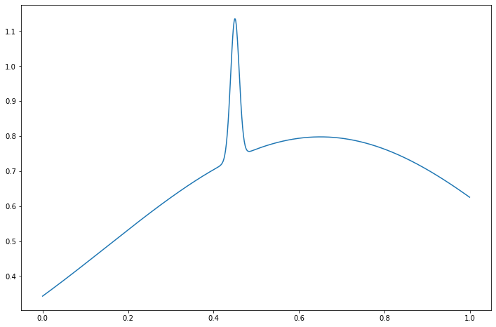
png
It’s hard to estimate \(f\) using the methods we discussed so far. If we use a cosine basis and only keep the low order terms, we will miss the peak; if we allow higher order terms we will find the peak but we will make the rest of the curve very wiggly. Similar comments apply to kernel regression: if we use a large bandwidth, then we will smooth out the peak; if we use a small bandwidth, then we will find the peak but we will make the rest of the curve very wiggly.
One way to estimate inhomogeneous functions is to use a more carefully chosen basis that allows us to place a “blip” in some small region without adding wiggles elsewhere. In this section, we describe a special class of bases called wavelets that are aimed at fixing this problem. Statistical inference using wavelets is a large and active area. We will just discuss a few ideas to get a flavor of this approach.
The father Haar wavelet of Haar scaling function is defined by
\[ \phi(x) = \begin{cases} 1 & \text{if } 0 \leq x < 1 \\ 0 & \text{otherwise} \end{cases} \]
The mother Haar wavelet is defined by
\[ \psi(x) = \begin{cases} -1 & \text{if } 0 \leq x \leq \frac{1}{2} \\ 1 & \text{if } \frac{1}{2} < x \leq 1 \end{cases} \]
For any integers \(j\) and \(k\) define
\[ \phi_{j, k}(x) = 2^{j/2} \phi(2^j x - k) \quad \text{and} \quad \psi_{j, k}(x) = 2^{j/2} \psi(2^j x - k) \]
The function \(\psi_{j, k}\) has the same shape as \(\psi\) but it has been rescaled by a factor of \(2^{j/2}\) and shifted by a factor of \(k\).
import numpy as np

def haar_father_wavelet(x):
    return np.where((x >= 0) & (x < 1), 1, 0)

def haar_mother_wavelet(x):
    return np.where((x >= 0) & (x < 1),  np.where(x <= 1/2, -1, 1), 0)

def phi_wavelet(j, k):
    def f(x):
        return 2**(j / 2) * haar_father_wavelet((2**j)*x - k)
    return f

def psi_wavelet(j, k):
    def f(x):
        return 2**(j / 2) * haar_mother_wavelet((2**j)*x - k)
    return f
import matplotlib.pyplot as plt
%matplotlib inline
step = 1e-4
xx = np.arange(-1, 2, step=step)
plt.figure(figsize=(12, 12))
ax = plt.subplot(3, 2, 1)
ax.plot(xx, haar_father_wavelet(xx))
ax.set_title(r'Father wavelet $\phi$')
ax = plt.subplot(3, 2, 2)
ax.plot(xx, haar_mother_wavelet(xx))
ax.set_title(r'Mother wavelet $\psi$')
ax = plt.subplot(3, 2, 3)
ax.plot(xx, phi_wavelet(2, 2)(xx))
ax.set_title(r'$\phi_{2, 2}$')
ax = plt.subplot(3, 2, 4)
ax.plot(xx, phi_wavelet(4, 2)(xx))
ax.set_title(r'$\phi_{4, 2}$')
ax = plt.subplot(3, 2, 5)
ax.plot(xx, psi_wavelet(4, 10)(xx))
ax.set_title(r'$\psi_{4, 10}$')
ax = plt.subplot(3, 2, 6)
ax.plot(xx, psi_wavelet(6, 10)(xx))
ax.set_title(r'$\psi_{6, 10}$')
plt.tight_layout()
plt.show()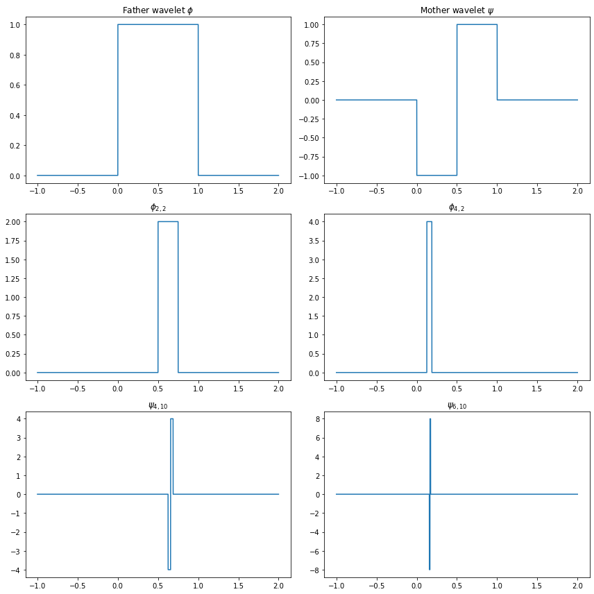
png
Notice that for large \(j\), \(\psi_{j, k}\) is a very localized function. This makes it possible to add a blip to a function without adding wiggles elsewhere. In technical terms, we say that wavelets provide a multiresolution analysis of \(L_2(0, 1)\).
Let
\[ W_j = \{\psi_{j, k}, \; k = 0, 1, \dots, 2^j - 1\} \] where \[\psi_{j, k}(x) = 2^{j/2} \psi(2^j x - k)\]
be the set of rescaled and shifted mother wavelets at resolution \(j\).
Theorem 22.13. The set of functions
\[ \left\{ \phi, W_0, W_1, W_2, \dots \right\} \]
is an orthonormal basis for \(L_2(0, 1)\).
It follows from this theorem that we can expand any function \(f \in L_2(0, 1)\) in this basis. Because each \(W_j\) is itself a set of functions, we write the expansion as a double sum:
\[ f(x) = \alpha \phi(x) + \sum_{j=0}^\infty \sum_{k=0}^{2^j - 1} \beta_{j, k} \psi_{j, k}(x) \]
where
\[ \alpha = \int_0^1 f(x) \phi(x) dx, \quad \beta_{j, k} = \int_0^1 f(x) \psi_{j, k}(x) dx\]
We call \(\alpha\) the scaling coefficient and \(\beta_{j, k}\) the detail coefficients. We call the finite sum
\[ \tilde{f}(x) = \alpha \phi(x) + \sum_{j=0}^{J - 1} \sum_{k=0}^{2^j - 1} \beta_{j, k}\psi_{j, k}(x)\]
the resolution \(J\) approximation to \(f\). The total number of terms in this sum is
\[ 1 + \sum_{j=0}^{J - 1}2^j = 2^J\]
Haar wavelets are localized, meaning they are zero outside of an interval, but they are not smooth. In 1988, Ingrid Daubechie showed that such wavelets do exist. They can be constructed numerically, but there is no closed form formula for smoother wavelets. To keep things simple, we will continue to use Haar wavelets.
We can now use wavelets to do density estimation and regression. We shall only discuss the regression problem \(Y_i = r(x_i) + \sigma \epsilon_i\) where \(\epsilon_i \sim N(0, 1)\) and \(x_i = i / n\). To simplify this discussion we assume that \(n = 2^J\) for some \(J\).
There is one major difference between estimation using wavelets instead of a cosine (or polynomial) basis. With the cosine basis, we used all terms \(1 \leq j \leq J\) for some \(J\). With wavelets, we use a method called thresholding where we keep a term in the function approximation only if its coefficient is large. The simplest version is called hard, universal thresholding.
Haar Wavelet Regression
- Let \(J = \log_2 n\) and define
\[ \hat{\alpha} = \frac{1}{n} \sum_i \phi(x_i) Y_i \quad \text{and} \quad D_{j, k} = \frac{1}{n} \sum_i \psi_{j, k}(x_i) Y_i \]
for \(0 \leq j \leq J - 1\)
- Estimate \(\sigma\) by
\[ \hat{\sigma} = \sqrt{n} \; \times \; \frac{\text{median} \left( \left| D_{J-1, k} : k = 0, \dots, 2^{J - 1} - 1\right| \right)}{0.6745} \]
- Apply universal thresholding:
\[ \hat{\beta}_{j, k} = \begin{cases} D_{j, k} & \text{if } \left| D_{j, k} \right| > \hat{\sigma} \sqrt{\frac{2 \log n}{n}} \\ 0 & \text{otherwise} \end{cases}\]
- Set
\[ \hat{f}(x) = \hat{\alpha} \phi(x) + \sum_{j = j_0}^{J - 1} \sum_{k = 0}^{2^j - 1} \hat{\beta}_{j, k} \psi_{j, k}(x) \]
In practice, we do not compute \(\hat{\alpha}\) and \(D_{j, k}\). Instead, we use the discrete wavelet transform (DWT) which is very fast. For Haar wavelets, the DWT works as follows.
DWT for Haar Wavelets
- Let \(y = (Y_1, \dots, Y_n)\) and let \(J = \log_2 n\).
- Create a list \(D\) with elements \(D[0], ..., D[J - 1]\)
- Do:
temp <- y / sqrt(n)
for j in (J - 1):0 {
  m <- 2^j
  I <- (1:m)
  D[j] <- (temp[2 * I] - temp[(2 * I) - 1]) / sqrt(2)
  temp <- (temp[2 * I] + temp[(2 * I) - 1]) / sqrt(2)
}
The estimate used for \(\sigma\) probably looks strange. It is similar to the estimate used for the cosine basis but it is designed to be insensitive to sharp peaks in the function.
To understand the intuition behind universal thresholding, consider what happens when there is no signal, that is, when \(\beta_{j, k} = 0\) for all \(j, k\).
Theorem 22.16. Suppose that \(\beta_{j, k} = 0\) for all \(j, k\) and let \(\hat{\beta}_{j, k}\) be the universal threshold estimator. Then
\[ \mathbb{P}\left(\hat{\beta}_{j, k} = 0 \; \text{for all } j, k \right) \rightarrow 1 \]
as \(n \rightarrow \infty\).
Proof Assume \(\sigma\) is known. Now \(D_{j, k} \approx N(0, \sigma^2 / n)\). We will need Mill’s inequality: if \(Z \sim N(0, 1)\) then \(\mathbb{P}(|Z| > t) \leq (c / t) e^{-t^2 / 2}\) where \(c = \sqrt{2 / pi}\) is a constant. Thus,
\[ \begin{align} \mathbb{P}(\max |D_{j, k}| > \lambda) &\leq \sum_{j, k} \mathbb{P}(|D_{j, k}| > \lambda) \\ & \leq \sum_{j, k} \mathbb{P} \left( \frac{\sqrt{n} |D_{j, k}|}{\sigma} > \frac{\sqrt{n} \lambda}{\sigma} \right) \\ & \leq \sum_{j, k} \frac{c \sigma}{\lambda \sqrt{n}} \exp \left\{ - \frac{1}{2} \frac{n \lambda^2}{\sigma^2} \right\} \\ & = \frac{c}{\sqrt{2 \log n}} \rightarrow 0 \end{align} \]
22.6 Exercises
Exercise 22.6.1. Prove Theorem 22.5.
The risk of \(\hat{f}\) is given by
\[ R(J) = \sum_{j=1}^J \frac{\sigma_j^2}{n} + \sum_{j=J+1}^\infty \beta_j^2 \]
Solution.
The density estimator \(\hat{f}\) is defined as
\[ \hat{f}(x) = \sum_{j=1}^J \hat{\beta}_j \phi_j(x) \quad \text{where} \quad \hat{\beta}_j = \frac{1}{n} \sum_{j=1}^n \phi_j(X_j)\]
From Theorem 22.4,
\[ \mathbb{E}[\hat{\beta}_j] = \beta_j \quad \text{and} \quad \mathbb{V}[\hat{\beta}_j] = \frac{\sigma_j^2}{n} \]
The (unintegrated) variance is
\[ \mathbb{V}[f(x) - \hat{f}(x)] = \mathbb{V}[\hat{f}(x)] = \mathbb{V}\left[\sum_{j=1}^J \hat{\beta}_j \phi_j(x)\right]\\ = \sum_{j=1}^J \mathbb{V}[\hat{\beta}_j]\phi_j(x)^2 + 2 \sum_{i < j} \text{Cov}(\hat{\beta}_i, \hat{\beta}_j) \phi_i(x) \phi_j(x) \]
so, integrating,
\[ \begin{align} \int \mathbb{V}[f(x) - \hat{f}(x)] dx &= \sum_{j=1}^J \mathbb{V}[\hat{\beta}_j] \int \phi_j(x)^2 dx + 2 \sum_{i < j} \text{Cov}(\hat{\beta}_i, \hat{\beta}_j) \int \phi_i(x) \phi_j(x) dx \\ &= \sum_{j=1}^J \mathbb{V}[\hat{\beta}_j] \langle \phi_j, \phi_j \rangle + 2 \sum_{i < j} \text{Cov}(\hat{\beta}_i, \hat{\beta}_j) \langle \phi_i, \phi_j \rangle \\ &= \sum_{j=1}^J \mathbb{V}[\hat{\beta}_j] = \sum_{j=1}^J \frac{\sigma_j^2}{n} \end{align} \]
while the integrated expected bias squared is:
\[ \begin{align} \int \mathbb{E}\left[\left(f(x) - \hat{f}(x)\right)^2\right] dx &= \int \mathbb{E}\left[\left(\sum_{j=1}^\infty \beta_j \phi_j(x) - \sum_{j=1}^J \hat{\beta}_j \phi_j(x)\right)^2\right] dx \\ &= \int \mathbb{E} \left[ \left(\sum_{j=1}^\infty \beta_j \phi_j(x)\right)^2 \right] dx + \int \mathbb{E} \left[ \left(\sum_{j=1}^J \hat{\beta}_j \phi_j(x)\right)^2 \right] dx - 2\int \mathbb{E} \left[ \sum_{i=1}^\infty \sum_{j=1}^J \beta_i \hat{\beta}_j \phi_i(x) \phi_j(x) \right] dx \\ &= \sum_{j=1}^\infty \beta_j^2 \int \phi_j(x)^2 dx + \sum_{j=1}^J \beta_j^2 \int \phi_j(x)^2 dx - 2 \sum_{j=1}^J \beta_j^2 \int \phi_j(x)^2 dx \\ &= \sum_{j=J+1}^\infty \beta_j^2 \end{align} \]
since \(\langle \phi_i, \phi_j \rangle = \int \phi_i(x) \phi_j(x) dx = 0\) for \(i \neq j\), and since \(\langle \phi_j, \phi_j \rangle = \int \phi_j(x)^2 dx = 1\).
Then, the risk is the bias squared plus the variance,
\[ R(J) = \sum_{j=1}^J \frac{\sigma_j^2}{n} + \sum_{j=J+1}^\infty \beta_j^2\]
as desired.
Exercise 22.6.2. Prove Theorem 22.9.
The risk \(R(J)\) of the estimator $ (x) = _{j=1}^J _j _j(x) $ is
\[ R(J) = \frac{J \sigma^2}{n} + \sum_{j=J+1}^\infty \beta_j^2 \]
Solution. Consider the probability distribution function obtained by shifting the true regression function to a minimum of 0, and rescaled to integrate to 1:
\[ f(x) = \frac{r(x) - r_0}{A} \quad \text{where } A = \int r(y) dy - r_0, r_0 = \inf_x r(x) \]
But if \(r(x) = \sum_{j=1}^\infty \beta_j \phi_j(x)\), then
\[ f(x) = -\frac{r_0}{A} + \sum_{j=1}^\infty \left( \frac{\beta_j}{A} \right) \phi_j(x) = \sum_{j=1}^\infty \left( \frac{\beta_j}{A} + c_j \right) \phi_j(x) \]
where the \(c_j\)’s are the decomposition of the constant function \(-r_0 / A\) on the basis of the functions \(\phi_j\)’s. Assuming a sensible basis, \(\phi_0\) is constant and \(c_j = 0\) for \(j > 1\).
By theorem 22.5, the risk of the PDF estimation is
\[ \sum_{j=1}^J \frac{\sigma_j^2}{A^2n} + \sum_{j=J+1}^\infty \left( \frac{\beta_j}{A} \right)^2 = \frac{1}{A^2} \left( \frac{J \sigma^2}{n} + \sum_{j=J+1}^\infty \beta_j^2 \right)\]
and so the result follows.
Exercise 22.6.3. Let
\[ \psi_1 = \left( \frac{1}{\sqrt{3}}, \frac{1}{\sqrt{3}} , \frac{1}{\sqrt{3}} \right), \quad \psi_2 = \left( \frac{1}{\sqrt{2}}, -\frac{1}{\sqrt{2}} , 0 \right), \quad \psi_3 = \left( \frac{1}{\sqrt{6}}, \frac{1}{\sqrt{6}} , -\frac{2}{\sqrt{6}} \right) \]
Show that these vectors have norm 1 and are orthogonal.
Solution. Results follow from inspection.
Norms:
\[ \begin{align} \langle \psi_1, \psi_1 \rangle &= \frac{1}{\sqrt{3}} \cdot \frac{1}{\sqrt{3}} + \frac{1}{\sqrt{3}} \cdot \frac{1}{\sqrt{3}} + \frac{1}{\sqrt{3}} \cdot \frac{1}{\sqrt{3}} \\&= \frac{1}{3} + \frac{1}{3} + \frac{1}{3} &= 1 \\ \langle \psi_2, \psi_2 \rangle &= \frac{1}{\sqrt{2}} \cdot \frac{1}{\sqrt{2}} + \frac{-1}{\sqrt{2}} \cdot \frac{-1}{\sqrt{2}} + 0 \cdot 0 \\&= \frac{1}{2} + \frac{1}{2} + 0 &= 1 \\ \langle \psi_3, \psi_3 \rangle &= \frac{1}{\sqrt{6}} \cdot \frac{1}{\sqrt{6}} + \frac{1}{\sqrt{6}} \cdot \frac{1}{\sqrt{6}} + \frac{-2}{\sqrt{6}} \cdot \frac{-2}{\sqrt{6}}\\ &= \frac{1}{6} + \frac{1}{6} + \frac{4}{6} &= 1 \end{align} \]
Orthogonality: \[ \begin{align} \langle \psi_1, \psi_2 \rangle &= \frac{1}{\sqrt{3}} \cdot \frac{1}{\sqrt{2}} + \frac{1}{\sqrt{3}} \cdot \frac{-1}{\sqrt{2}} + \frac{1}{\sqrt{3}} \cdot 0 \\&= \frac{1}{\sqrt{6}} + \frac{-1}{\sqrt{6}} + 0 &= 0 \\ \langle \psi_1, \psi_3 \rangle &= \frac{1}{\sqrt{3}} \cdot \frac{1}{\sqrt{6}} + \frac{1}{\sqrt{3}} \cdot \frac{1}{\sqrt{6}} + \frac{1}{\sqrt{3}} \cdot \frac{-2}{\sqrt{6}} \\&= \frac{1}{3\sqrt{2}} + \frac{1}{3\sqrt{2}} + \frac{-2}{3\sqrt{2}} &= 0 \\ \langle \psi_2, \psi_3 \rangle &= \frac{1}{\sqrt{2}} \cdot \frac{1}{\sqrt{6}} + \frac{-1}{\sqrt{2}} \cdot \frac{1}{\sqrt{6}} + 0 \cdot \frac{-2}{\sqrt{6}} \\&= \frac{1}{2\sqrt{3}} + \frac{-1}{2\sqrt{3}} + 0 &= 0 \end{align} \]
Exercise 22.6.4. Prove Parseval’s relation equation.
\[ \Vert f \Vert^2 \equiv \int f^2(x) dx = \sum_{j=1}^\infty \beta_j^2 \equiv \Vert \beta \Vert^2\]
Solution. We have:
\[ \begin{align} \int f^2(x) dx &= \int \left( \sum_{i=1}^\infty \beta_i \phi_i(x) \right)^2 dx \\ &= \int \left( \sum_{i=1}^\infty \beta_i^2 \phi_i^2(x) + \sum_{i=1}^\infty \sum_{j=1, j \neq i}^\infty \beta_i \beta_j \phi_i(x) \phi_j(x) \right) dx \\ &= \sum_{i=1}^\infty \beta_i^2 \int \phi_i^2(x) dx + \sum_{i=1}^\infty \sum_{j=1, j \neq i}^\infty \beta_i \beta_j \int \phi_i(x) \phi_j(x) dx \\ &= \sum_{i=1}^\infty \beta_i^2 \langle \phi_i, \phi_i \rangle + \sum_{i=1}^\infty \sum_{j=1, j \neq i}^\infty \beta_i \beta_j \langle \phi_i, \phi_j \rangle \\ &= \sum_{i=1}^\infty \beta_i^2 \end{align} \]
since \(\langle \phi_i, \phi_i \rangle = 1\) and \(\langle \phi_i, \phi_j \rangle = 0\) for \(i \neq j\).
Exercise 22.6.5. Plot the first five Legendre polynomials. Verify, numerically, that they are orthonormal.
The Legendre polynomials on \([-1, 1]\) are defined by
\[ P_j(x) = \frac{1}{2^j j!} \frac{d^j}{dx^j} (x^2 - 1)^j, \quad j = 0, 1, 2, \dots \]
It can be shown that these functions are complete and orthogonal, and that
\[ \int_{-1}^1 P_j^2(x) dx = \frac{2}{2j + 1}\]
It follows that the functions
\[ \phi_j(x) = \sqrt{\frac{2j + 1}{2}}P_j(x), \quad j = 0, 1, 2, \dots \]
form an orthonormal basis for \(L_2[-1, 1]\). The first few Legendre polynomials are
\[ \begin{align} P_0(x) &= 1 \\ P_1(x) &= x \\ P_2(x) &= \frac{1}{2}\left( 3x^2 - 1 \right) \\ P_3(x) &= \frac{1}{2}\left( 5x^3 - 3x \right) \end{align} \]
These polynomials may be constructed explicitly using the following recursive relation:
\[ P_{j+1}(x) = \frac{(2j + 1) x P_j(x) - j P_{j - 1}(x)}{j + 1} \]
Solution.
import sympy
from sympy.abc import x
from functools import lru_cache

@lru_cache(maxsize=None)
def legendre_polynomial(j):
    if j == 0:
        return 1
    if j == 1:
        return x

    return sympy.expand(((2*j - 1) * x * legendre_polynomial(j - 1) - (j - 1) * legendre_polynomial(j - 2)) / j)

def legendre_basis(j):
    if j == 0:
        return lambda x: np.sqrt(1/2) * np.ones_like(x)

    pj = legendre_polynomial(j)
    return sympy.lambdify(x, sympy.sqrt((2*j + 1) / 2) * pj, "numpy")
import matplotlib.pyplot as plt
%matplotlib inline
step = 1e-4
xx = np.arange(-1, 1 + step, step=step)
plt.figure(figsize=(12, 12))
for i in range(0, 5):
# Set up the plot
ax = plt.subplot(5, 1, i + 1)
ax.plot(xx, legendre_basis(i)(xx))
ax.set_title(r'Legendre Basis $\phi_%i$' % i)
plt.tight_layout()
plt.show()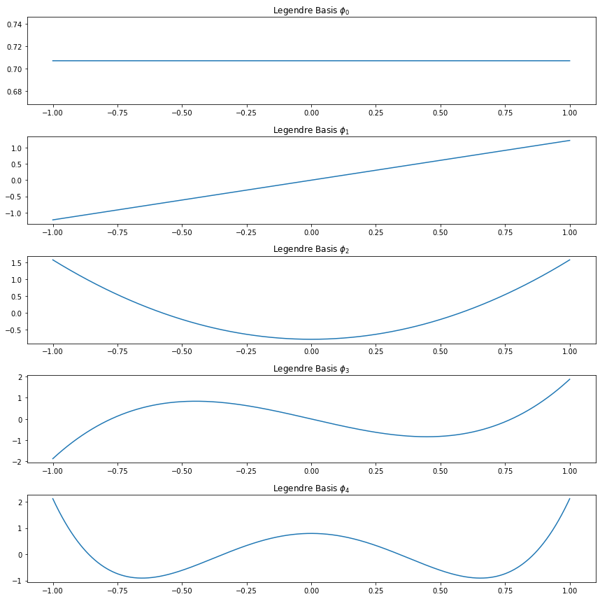
png
# Verifying orthogonality numerically

for i in range(0, 5):
    for j in range(i,5):
        product = legendre_basis(i)(xx) @ legendre_basis(j)(xx) * step
        print("<phi_%i, phi_%i>: %.3f" % (i, j, product))
<phi_0, phi_0>: 1.000
<phi_0, phi_1>: -0.000
<phi_0, phi_2>: 0.000
<phi_0, phi_3>: -0.000
<phi_0, phi_4>: 0.000
<phi_1, phi_1>: 1.000
<phi_1, phi_2>: -0.000
<phi_1, phi_3>: 0.000
<phi_1, phi_4>: -0.000
<phi_2, phi_2>: 1.000
<phi_2, phi_3>: -0.000
<phi_2, phi_4>: 0.000
<phi_3, phi_3>: 1.000
<phi_3, phi_4>: -0.000
<phi_4, phi_4>: 1.000Exercise 22.6.6. Expand the following functions in the cosine basis on \([0, 1]\). For (a) and (b), find the coefficients \(\beta_j\) analytically. For (c) and (d), find the coefficients \(\beta_j\) numerically, i.e.
\[ \beta_j = \int_0^1 f(x) \phi_j(x) \approx \frac{1}{N} \sum_{r=1}^N f \left( \frac{r}{N} \right) \phi_j \left( \frac{r}{N} \right) \]
for some large integer \(N\). Then plot the partial sum \(\sum_{j=1}^n \beta_j \phi_j(x)\) for increasing values of \(n\).
(a) \(f(x) = \sqrt{2} \cos (3 \pi x)\)
(b) \(f(x) = \sin(\pi x)\)
(c) \(f(x) = \sum_{j=1}^{11} h_j K(x - t_j)\), where \(K(t) = (1 + \text{sign}(t)) / 2\),
\[ (t_j) = (.1, .13, .15, .23, .25, .40, .44, .65, .76, .78, .81), \\ (h_j) = (4, -5, 3, -4, 5, -4.2, 2.1, 4.3, -3.1, 2.1, -4.2) \]
(d) \[f(x) = \sqrt{x(1-x)} \sin \left( \frac{2.1 \pi}{(x + .05)} \right) \]
Solution.
(a) is immediate by inspection:
\[ f(x) = \sqrt{2} \cos(3 \pi x) = \sum_{j=1}^\infty \beta_j \phi_j(x), \quad \text{where } \phi_j(x) = \sqrt{2} \cos((j - 1) \pi x) \]
so
\[ \beta_j = \begin{cases} 1 & \text{if } j = 4 \\ 0 & \text{otherwise} \end{cases} \]
import numpy as np

def beta_j(j):
    if j == 4:
        return 1
    return 0

def phi_j(j):
    def f(x):
        if j == 1:
            return np.ones_like(x)
        return np.sqrt(2) * np.cos((j - 1) * np.pi * x)
    return f

def partial_sum(n, x):
    lx = len(x)
    terms = np.empty((n, lx))
    for j in range(1, n + 1):
        terms[j - 1] = beta_j(j) * phi_j(j)(xx)
    return terms.sum(axis = 0)
# Plot in separate boxes for ease of visualization
import matplotlib.pyplot as plt
%matplotlib inline
step = 1e-4
xx = np.arange(0, 1 + step, step=step)
plt.figure(figsize=(12, 12))
def do_subplot(index, xx, yy, label, color):
ax = plt.subplot(4, 1, index)
ax.plot(xx, yy, label=label, color=color)
ax.legend()
do_subplot(1, xx, partial_sum(3, xx), label=r'$n \leq 3$', color='C0')
do_subplot(2, xx, partial_sum(4, xx), label=r'$n \geq 4$', color='C2')
do_subplot(3, xx, partial_sum(4, xx), label=r'$f(x) = \sqrt{2} \cos (3 \pi x)$', color='C3')
do_subplot(4, xx, partial_sum(5, xx), label=r'$n = 5$', color='C4')
plt.tight_layout()
plt.legend()
plt.show()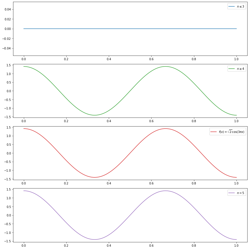
png
(b) can be solved with the definition of \(\beta_j\):
For \(j = 1\),
\[ \beta_j = \langle f, \phi_1 \rangle = \int_0^1 f(x) \phi_1(x) dx = \int_0^1 \sin(\pi x) dx = \frac{2}{\pi} \]
For \(j \geq 2\),
\[ \beta_j = \langle f, \phi_j \rangle = \int_0^1 f(x) \phi_j(x) dx = \int_0^1 \sin(\pi x) \left( \sqrt{2} \cos((j-1) \pi x) \right) dx = \frac{\sqrt{2} (\cos(\pi j) - 1)}{\pi j^2 - 2 \pi j } \]
so
\[ \beta_j = \begin{cases} \frac{2}{\pi} & \text{if } j = 1\\ -\frac{2\sqrt{2}}{\pi j^2 - 2 \pi j} & \text{if } j \text{ is odd}, j > 1 \\ 0 & \text{if } j \text{ is even} \end{cases} \]
import numpy as np

def beta_j(j):
    if j % 2 == 0:
        return 0
    if j == 1:
        return 2 / np.pi
    return -np.sqrt(2)*2 / ((np.pi * j * j) - (2 * np.pi * j))

def phi_j(j):
    def f(x):
        if j == 1:
            return np.ones_like(x)
        return np.sqrt(2) * np.cos((j - 1) * np.pi * x)
    return f

def partial_sum(n, x):
    lx = len(x)
    terms = np.empty((n, lx))
    for j in range(1, n + 1):
        terms[j - 1] = beta_j(j) * phi_j(j)(xx)
    return terms.sum(axis = 0)
# Plot in separate boxes for ease of visualization
import matplotlib.pyplot as plt
%matplotlib inline
step = 1e-4
xx = np.arange(0, 1 + step, step=step)
plt.figure(figsize=(12, 12))
def do_subplot(index, xx, yy, label, color):
ax = plt.subplot(4, 1, index)
ax.plot(xx, yy, label=label, color=color)
ax.legend()
do_subplot(1, xx, partial_sum(4, xx), label=r'$n = %i$' % 4, color='C0')
do_subplot(2, xx, partial_sum(8, xx), label=r'$n = %i$' % 8, color='C1')
do_subplot(3, xx, partial_sum(16, xx), label=r'$n = %i$' % 16, color='C2')
do_subplot(4, xx, np.sin(np.pi * xx), label=r'$f(x) = \sin(\pi x)$', color='C3')
plt.tight_layout()
plt.legend()
plt.show()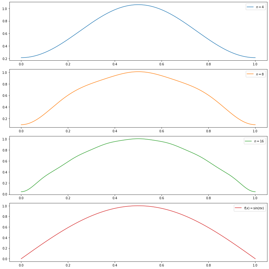
png
(c)
\[f(x) = \sum_{j=1}^{11} h_j K(x - t_j)\] where \(K(t) = (1 + \text{sign}(t)) / 2\),
\[ (t_j) = (.1, .13, .15, .23, .25, .40, .44, .65, .76, .78, .81), \\ (h_j) = (4, -5, 3, -4, 5, -4.2, 2.1, 4.3, -3.1, 2.1, -4.2) \]
import numpy as np

T = np.array([.1, .13, .15, .23, .25, .40, .44, .65, .76, .78, .81])
H = np.array([4, -5, 3, -4, 5, -4.2, 2.1, 4.3, -3.1, 2.1, -4.2])

def phi_j(j):
    def f(x):
        if j == 1:
            return np.ones_like(x)
        return np.sqrt(2) * np.cos((j - 1) * np.pi * x)
    return f

def f(x):
    def K(t):
        return (1 + np.sign(t))/2
    # reshape(1, -1) change to 1 row array, the unspecified value is inferred to be len(x)
    return (H.reshape(1, -1) * K(
        x.reshape(-1, 1).repeat(len(T), axis=1) - T.reshape(-1, 1).repeat(len(x), axis=1).T)
    ).sum(axis = 1)
N = 10000
step = 1 / N
xx = np.arange(0, 1 + step, step=step)
J = 256
estimated_beta = np.empty(J)
for j in range(1, J + 1):
estimated_beta[j - 1] = f(xx) @ phi_j(j)(xx) / N
def beta_j(j):
return estimated_beta[j - 1]
def partial_sum(n, x):
lx = len(x)
terms = np.empty((n, lx))
for j in range(1, n + 1):
terms[j - 1] = beta_j(j) * phi_j(j)(xx)
return terms.sum(axis = 0)# Plot in separate boxes for ease of visualization
import matplotlib.pyplot as plt
%matplotlib inline
step = 1e-4
xx = np.arange(0, 1 + step, step=step)
plt.figure(figsize=(12, 12))
def do_subplot(index, xx, yy, label, color):
ax = plt.subplot(4, 1, index)
ax.plot(xx, yy, label=label, color=color)
ax.legend()
do_subplot(1, xx, partial_sum(16, xx), label=r'$n = %i$' % 16, color='C0')
do_subplot(2, xx, partial_sum(64, xx), label=r'$n = %i$' % 64, color='C1')
do_subplot(3, xx, partial_sum(256, xx), label=r'$n = %i$' % 256, color='C2')
do_subplot(4, xx, f(xx), label=r'$f(x) = \sum_j h_j K(x - t_j) $', color='C3')
plt.tight_layout()
plt.legend()
plt.show()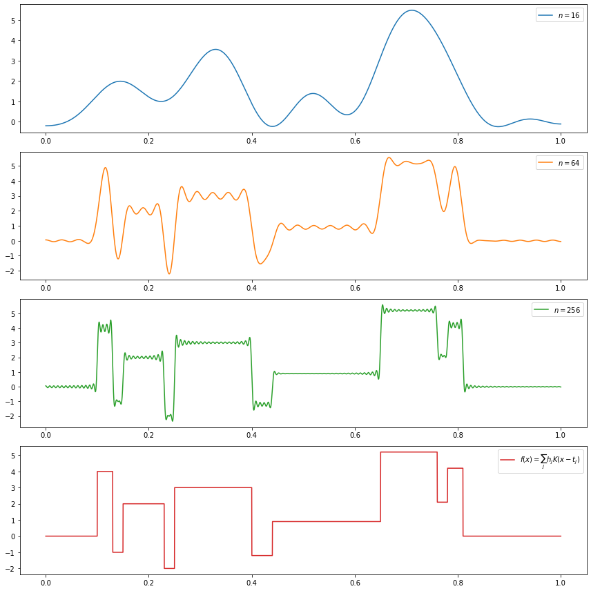
png
(d)
\[f(x) = \sqrt{x(1-x)} \sin \left( \frac{2.1 \pi}{(x + .05)} \right) \]
import numpy as np

def phi_j(j):
    def f(x):
        if j == 1:
            return np.ones_like(x)
        return np.sqrt(2) * np.cos((j - 1) * np.pi * x)
    return f

def f(x):
    return np.sqrt(x * (1 - x)) * np.sin(2.1 * np.pi / (x + 0.05))
N = 10000
step = 1 / N
xx = np.arange(0, 1 + step, step=step)
J = 512
estimated_beta = np.empty(J)
for j in range(1, J + 1):
estimated_beta[j - 1] = f(xx) @ phi_j(j)(xx) / N
def beta_j(j):
return estimated_beta[j - 1]
def partial_sum(n, x):
lx = len(x)
terms = np.empty((n, lx))
for j in range(1, n + 1):
terms[j - 1] = beta_j(j) * phi_j(j)(xx)
return terms.sum(axis = 0)# Plot in separate boxes for ease of visualization
import matplotlib.pyplot as plt
%matplotlib inline
step = 1e-4
xx = np.arange(0, 1 + step, step=step)
plt.figure(figsize=(12, 12))
def do_subplot(index, xx, yy, label, color):
ax = plt.subplot(4, 1, index)
ax.plot(xx, yy, label=label, color=color)
ax.legend()
do_subplot(1, xx, partial_sum(16, xx), label=r'$n = %i$' % 16, color='C0')
do_subplot(2, xx, partial_sum(64, xx), label=r'$n = %i$' % 64, color='C1')
do_subplot(3, xx, partial_sum(512, xx), label=r'$n = %i$' % 512, color='C2')
do_subplot(4, xx, f(xx), label=r'$f(x) = \sqrt{x (1 - x)} \sin \left( \frac{2.1 \pi}{(x + .05)} \right)$', color='C3')
plt.tight_layout()
plt.legend()
plt.show()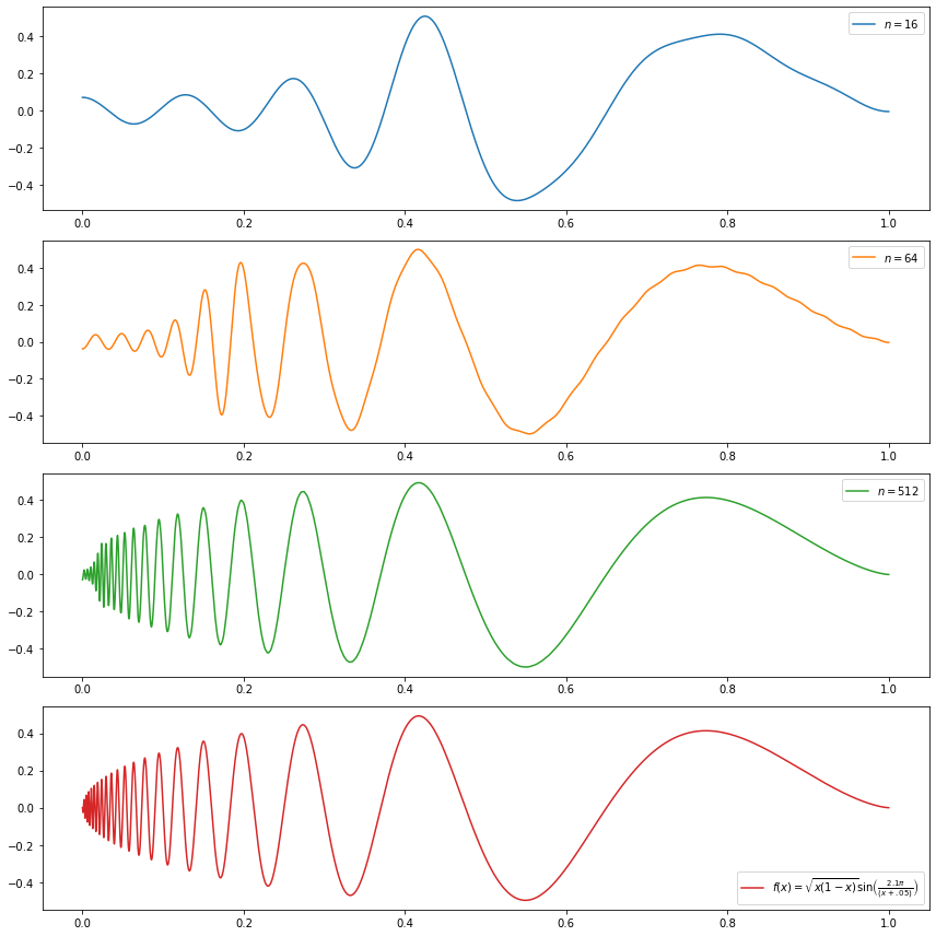
png
Exercise 22.6.7. Consider the glass fragments data. Let \(Y\) be the refractive index and let \(X\) be aluminium content (the fourth variable).
(a) Do a nonparametric regression to fit the model \(Y = f(x) + \epsilon\) using the cosine basis method. The data are not on a regular grid. Ignore this when estimating the function. (But do sort the data first.) Provide a function estimate, an estimate of the risk, and a confidence band.
(b) Use the wavelet method to estimate \(f\).
Solution.
import numpy as np
import pandas as pd

data = pd.read_csv('data/glass.txt', delim_whitespace=True)
data = data[['Al', 'RI']].sort_values(by='Al', ignore_index=True)
X, Y = data['Al'], data['RI']
data| Al | RI | |
|---|---|---|
| 0 | 0.29 | 1.66 |
| 1 | 0.34 | -6.85 |
| 2 | 0.47 | 4.13 |
| 3 | 0.47 | 4.13 |
| 4 | 0.51 | 5.20 |
| … | … | … |
| 209 | 2.79 | -1.77 |
| 210 | 2.88 | -1.77 |
| 211 | 3.02 | -4.79 |
| 212 | 3.04 | -4.84 |
| 213 | 3.50 | -2.86 |
214 rows × 2 columns
(a)
Orthogonal Series Regression Estimator
- Let
\[ \hat{\beta}_j = \frac{1}{n} \sum_{i=1}^n Y_i \phi_i(x_i), \quad j = 1, \dots, n\]
- Let
\[ \hat{\sigma}^2 = \frac{n}{k} \sum_{i=n-k+1}^n \hat{\beta}_j^2 \]
where \(k \approx n / 4\).
- For \(1 \leq J \leq n\), compute the risk estimate
\[ \hat{R}(J) = J \frac{\hat{\sigma}^2}{n} + \sum_{j=J+1}^n \left(\hat{\beta}_j^2 - \frac{\hat{\sigma}^2}{n} \right)_{+} \]
Choose \(\hat{J} \in \{1, \dots, n \}\) to minimize \(\hat{R}(J)\).
Let
\[ \hat{f}(x) = \sum_{j=1}^J \hat{\beta}_j \phi_j(x) \]
Theorem 22.11. Suppose the estimate \(\hat{r}\) is based on \(J\) terms and $^2 = _{i=n-k+1}^n _j^2 $. Assume that \(J < n - k + 1\). An approximate \(1 - \alpha\) confidence band for \(\overline{r}\) is \((\ell, u)\), where
\[ \ell(x) = \hat{r}(x) - K \sqrt{J} \sqrt{\frac{z_{\alpha} \hat{\tau}}{\sqrt{n}} + \frac{J \hat{\sigma}^2}{n}} \quad \text{and} \quad u(x) = \hat{r}(x) + K \sqrt{J} \sqrt{\frac{z_{\alpha} \hat{\tau}}{\sqrt{n}} + \frac{J \hat{\sigma}^2}{n}} \]
where
\[ K = \max_{1 \leq j \leq J} \max_x | \phi_j(x) | \]
and
\[ \hat{\tau}^2 = \frac{2 J \hat{\sigma}^4}{n} \left( 1 + \frac{J}{k} \right) \]
and \(k = n / 4\) as used in the definition of \(\hat{\sigma}^2\). In the cosine basis, \(K = \sqrt{2}\).
# Cosine basis function
def phi_j(j):
    def f(x):
        if j == 1:
            return np.ones_like(x)
        return np.sqrt(2) * np.cos((j - 1) * np.pi * x)
    return f
from scipy.stats import norm
def estimate_r(X, Y, alpha=0.05):
n = len(X)
# Rescale from [X.min(), X.max()] to [0, 1]
def X_to_L2(t):
return (t - X.min()) / (X.max() - X.min())
X_scaled = X_to_L2(X)
beta_hat = np.empty(n)
for j in range(1, n+1):
beta_hat[j - 1] = np.sum(Y @ phi_j(j)(X_scaled)) / n
k = int(np.ceil(n / 4))
sigma2_hat = np.sum(beta_hat[-k:]**2) * (n / k)
risk_hat = np.zeros(n)
for J in range(1, n + 1):
risk_hat[J - 1] = J * sigma2_hat/n + np.sum(np.maximum(beta_hat[J:]**2 - sigma2_hat/n, 0))
def r_hat(x):
xx = X_to_L2(x)
result = np.zeros_like(xx)
for j in range(1, J_hat):
result += beta_hat[j - 1] * phi_j(j)(xx)
return result
J_hat = np.argmin(risk_hat) + 2
tau_hat = sigma2_hat * np.sqrt((2 * J_hat / n) * (1 + J_hat / k))
z_alpha = norm.ppf(1 - alpha / 2)
c = np.sqrt(2 * J * ((z_alpha * tau_hat / np.sqrt(n)) + (J_hat * sigma2_hat / n)))
def r_lower(x):
return r_hat(x) - c
def r_upper(x):
return r_hat(x) + c
return r_hat, r_lower, r_upperr_hat, r_lower, r_upper = estimate_r(X, Y, alpha=0.05)import matplotlib.pyplot as plt
%matplotlib inline
plt.figure(figsize=(12, 8))
plt.scatter(X, Y, color='C0', marker='x', label='Data')
X_min, X_max = X.min(), X.max()
t = np.arange(X_min, X_max, step=(X_max - X_min) / 1000)
plt.plot(t, r_hat(t), color='purple', label='$\hat{r}(x)$')
plt.plot(t, r_lower(t), color='red', alpha=0.5, label='95% lower bound')
plt.plot(t, r_upper(t), color='green', alpha=0.5, label='95% upper bound')
plt.xlabel('Al content')
plt.ylabel('Refractive Index')
plt.legend()
plt.show()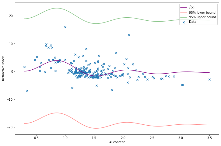
png
(b)
Haar Wavelet Regression
- Let \(J = \log_2 n\) and define
\[ \hat{\alpha} = \frac{1}{n} \sum_i \phi(x_i) Y_i \quad \text{and} \quad D_{j, k} = \frac{1}{n} \sum_i \psi_{j, k}(x_i) Y_i \]
for \(0 \leq j \leq J - 1\)
- Estimate \(\sigma\) by
\[ \hat{\sigma} = \sqrt{n} \; \times \; \frac{\text{median} \left( \left| D_{J-1, k} : k = 0, \dots, 2^{J - 1} - 1\right| \right)}{0.6745} \]
- Apply universal thresholding:
\[ \hat{\beta}_{j, k} = \begin{cases} D_{j, k} & \text{if } \left| D_{j, k} \right| > \hat{\sigma} \sqrt{\frac{2 \log n}{n}} \\ 0 & \text{otherwise} \end{cases}\]
- Set
\[ \hat{f}(x) = \hat{\alpha} \phi(x) + \sum_{j = j_0}^{J - 1} \sum_{k = 0}^{2^j - 1} \hat{\beta}_{j, k} \psi_{j, k}(x) \]
# Wavelet base functions

import numpy as np

def haar_father_wavelet(x):
    return np.where((x >= 0) & (x < 1), 1, 0)

def haar_mother_wavelet(x):
    return np.where((x >= 0) & (x < 1),  np.where(x <= 1/2, -1, 1), 0)

def psi_wavelet(j, k):
    def f(x):
        return 2**(j / 2) * haar_mother_wavelet((2**j)*x - k)
    return f
def estimate_r(X, Y):
n = len(Y)
J = int(np.ceil(np.log2(n)))
def X_to_L2(t):
return (t - X.min()) / (X.max() - X.min())
xx = X_to_L2(X)
alpha_hat = np.sum(Y) / n
D = {}
for j in range(J):
D[j] = np.zeros(2**j)
for k in range(2**j):
D[j][k] = psi_wavelet(j, k)(xx) @ Y / n
sigma_hat = np.sqrt(n) * np.median(np.abs(D[J - 1])) / 0.6745
threshold = sigma_hat * np.sqrt(2 * np.log(n) / n)
beta_hat = [(j, k, v) for j, values in D.items() for k, v in enumerate(values) if np.abs(v) > threshold]
def r_hat(X):
xx = X_to_L2(X)
return alpha_hat * haar_father_wavelet(xx) \
+ np.sum(np.array([v * psi_wavelet(j, k)(xx) for j, k, v in beta_hat]), axis=0)
return r_hatr_hat = estimate_r(X, Y)import matplotlib.pyplot as plt
%matplotlib inline
plt.figure(figsize=(12, 8))
plt.scatter(X, Y, color='C0', marker='x', label='Data')
X_min, X_max = X.min(), X.max()
t = np.arange(X_min, X_max, step=(X_max - X_min) / 10000)
plt.plot(t, r_hat(t), color='purple', label='$\hat{r}(x)$')
plt.xlabel('Al content')
plt.ylabel('Refractive Index')
plt.legend()
plt.show()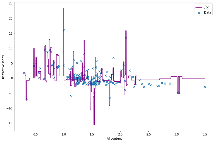
png
Exercise 22.6.8. Show that the Haar wavelets are orthonormal.
Solution.
Recalling the definitions:
The father Haar wavelet of Haar scaling function is defined by
\[ \phi(x) = \begin{cases} 1 & \text{if } 0 \leq x < 1 \\ 0 & \text{otherwise} \end{cases} \]
The mother Haar wavelet is defined by
\[ \psi(x) = \begin{cases} -1 & \text{if } 0 \leq x \leq \frac{1}{2} \\ 1 & \text{if } \frac{1}{2} < x \leq 1 \end{cases} \]
For any integers \(j\) and \(k\) define
\[ \phi_{j, k}(x) = 2^{j/2} \phi(2^j x - k) \quad \text{and} \quad \psi_{j, k}(x) = 2^{j/2} \psi(2^j x - k) \]
The function \(\psi_{j, k}\) has the same shape as \(\psi\) but it has been rescaled by a factor of \(2^{j/2}\) and shifted by a factor of \(k\) and increased frequency by a factor of \(2^j\).
Let
\[ W_j = \{\psi_{j, k}, \; k = 0, 1, \dots, 2^j - 1\} \]
be the set of rescaled and shifted mother wavelets at resolution \(j\).
Theorem 22.13. The set of functions
\[ \left\{ \phi, W_0, W_1, W_2, \dots \right\} \]
is an orthonormal basis for \(L_2(0, 1)\).
Proof.
Normality:
\[ \begin{align} \langle \phi, \phi \rangle &= \int_0^1 \phi^2(x) dx = \int_0^1 1 \; dx = 1 \\ \langle \psi_{j, k}, \psi_{j, k} \rangle &= \int_0^1 \psi_{j, k}^2(x) dx \\ &= \int_0^1 \left( 2^{j / 2} \psi(2^j x - k) \right)^2 dx \\ &= \int_{-k}^{2^j - k} 2^j \psi^2(y) \left( 2^{-j} dy \right) \\ &= \int_0^1 1 \; dy = 1 \end{align} \]
Orthogonality:
\[ \begin{align} \langle \phi, \psi_{j, k} \rangle &= \int_0^1 \phi(x) \psi_{j, k}(x) dx \\ &= \int_0^1 2^{j / 2} \psi(2^j x - k) dx \\ &= \int_{-k}^{2^j - k} 2^{j / 2} \psi(y) \left( 2^{-j} dy \right) \\ &= 2^{-j/2} \int_0^1 \psi(y) dy = 0 \end{align} \]
since \(\psi(y)\) has values \(-1\) for \(y \in [0, 1/2]\) and \(1\) for \([1/2, 1]\), and 0 otherwise, and \([0, 1] \subset [-k, 2^j - k]\).
\[ \begin{align} \langle \psi_{a, b}, \psi_{c, d} \rangle &= \int_0^1 \psi_{a, b}(x) \psi_{c, d}(x) \end{align} \]
For each wavelet \(\psi_{j, k}\), consider the domain of values that produce a non-zero function output,
\[F_{j, k} = \{ x : \psi_{j, k}(x) \neq 0 \} = \left[\frac{k}{2^j}, \frac{k + 1}{2^j} \right]\]
Also consider the regions that produce +1 and -1 outputs,
\[F_{j, k}^+ = \{ x : \psi_{j, k}(x) = 1 \} = \left[\frac{k + \frac{1}{2}}{2^j}, \frac{k + 1}{2^j} \right] \quad \text{and} \quad F_{j, k}^- = \{ x : \psi_{j, k}(x) = 1 \} = \left[\frac{k}{2^j}, \frac{k + \frac{1}{2}}{2^j} \right]\]
If \(a = c\), \(b \neq d\), then the non-zero domain of the wavelets do not overlap – each increment or decrement in the second parameter ‘shifts’ the whole non-zero domain by its size, i.e. the diameter of \(F_{j, k}\) which is \(2^{-j}\). Therefore, in this case, the integral is zero.
If \(a \neq c\), assuming without loss of generality \(a < c\), then we may have intersection in the non-zero areas. But in that case, the non-zero domain is fully contained within the plus or minus domain, \(F_{c, d} \subset F_{a, b}^+\) or \(F_{c, d} \subset F_{a, b}^-\). Therefore, in this case, the integral must also be zero.
Since we covered all cases, we have shown orthogonality. Since we have orthogonality and normality, the basis is orthonormal, proving the theorem.
Exercise 22.6.9. Consider again the doppler signal:
\[ f(x) = \sqrt{x (1 - x)} \sin \left( \frac{2.1 \pi}{x + 0.05} \right) \]
Let \(n = 1024\) and let \((x_1, \dots, x_n) = (1/n, \dots, 1)\). Generate data
\[ Y_i = f(x_i) + \sigma \epsilon_i \]
where \(\epsilon_i \sim N(0, 1)\).
(a) Fit the curve using the cosine basis method. Plot the function estimate and confidence band for \(J = 10, 20, \dots, 100\).
(b) Use Haar wavelets to fit the curve.
Solution. Let’s pick \(\sigma = 0.1\) when generating the data:
import numpy as np
from scipy.stats import norm

def f(x):
    return np.sqrt(x * (1 - x)) * np.sin( (2.1 * np.pi) / (x + 0.05) )

n = 1024
sigma = 0.1
X = np.arange(1, n + 1) / n
Y = f(X) + norm.rvs(loc=0, scale=sigma, size=n)
import matplotlib.pyplot as plt
%matplotlib inline
plt.figure(figsize=(12, 8))
plt.scatter(X, Y, marker='x')
plt.show()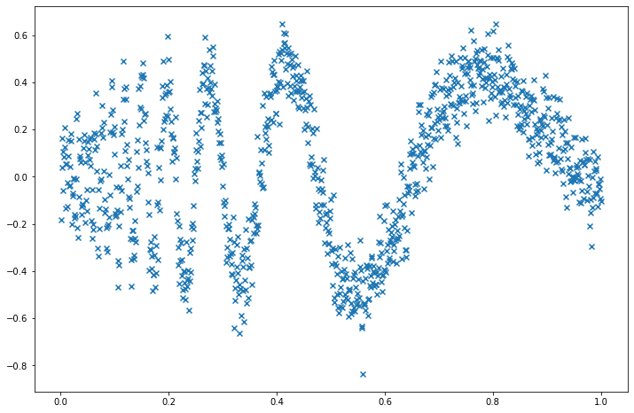
png
(a)
The cosine basis is defined as follows: Let \(\phi_1(x) = 1\) and for \(j \geq 2\) define
\[\phi_j(x) = \sqrt{2} \cos \left( (j - 1) \pi x\right)\]
\[ f(x) = \sum_{j=1}^\infty \beta_j \phi_j(x) \quad \text{where } \beta_j = \int_a^b f(x) \phi_j(x) dx \]
\[ Y_i = f(x_i) + \sigma \epsilon_i \text{ where }\epsilon_i \sim N(0, 1) \]
Orthogonal Series Regression Estimator
- Let
\[ \hat{\beta}_j = \frac{1}{n} \sum_{i=1}^n Y_i \phi_i(x_i), \quad j = 1, \dots, n\]
- Let
\[ \hat{\sigma}^2 = \frac{n}{k} \sum_{i=n-k+1}^n \hat{\beta}_j^2 \]
where \(k \approx n / 4\).
- For \(1 \leq J \leq n\), compute the risk estimate
\[ \hat{R}(J) = J \frac{\hat{\sigma}^2}{n} + \sum_{j=J+1}^n \left(\hat{\beta}_j^2 - \frac{\hat{\sigma}^2}{n} \right)_{+} \]
Choose \(\hat{J} \in \{1, \dots, n \}\) to minimize \(\hat{R}(J)\).
Let
\[ \hat{f}(x) = \sum_{j=1}^J \hat{\beta}_j \phi_j(x) \]
Theorem 22.11. Suppose the estimate \(\hat{r}\) is based on \(J\) terms and $^2 = _{i=n-k+1}^n _j^2 $. Assume that \(J < n - k + 1\). An approximate \(1 - \alpha\) confidence band for \(\overline{r}\) is \((\ell, u)\), where
\[ \ell(x) = \hat{r}(x) - K \sqrt{J} \sqrt{\frac{z_{\alpha} \hat{\tau}}{\sqrt{n}} + \frac{J \hat{\sigma}^2}{n}} \quad \text{and} \quad u(x) = \hat{r}(x) + K \sqrt{J} \sqrt{\frac{z_{\alpha} \hat{\tau}}{\sqrt{n}} + \frac{J \hat{\sigma}^2}{n}} \]
where
\[ K = \max_{1 \leq j \leq J} \max_x | \phi_j(x) | \]
and
\[ \hat{\tau}^2 = \frac{2 J \hat{\sigma}^4}{n} \left( 1 + \frac{J}{k} \right) \]
and \(k = n / 4\) as used in the definition of \(\hat{\sigma}^2\). In the cosine basis, \(K = \sqrt{2}\).
# Cosine basis function
def phi_j(j):
    def f(x):
        if j == 1:
            return np.ones_like(x)
        return np.sqrt(2) * np.cos((j - 1) * np.pi * x)
    return f
from scipy.stats import norm
def estimate_r(X, Y, J=None, alpha=0.05):
n = len(X)
# Rescale from [X.min(), X.max()] to [0, 1]
def X_to_L2(t):
return (t - X.min()) / (X.max() - X.min())
X_scaled = X_to_L2(X)
beta_hat = np.empty(n)
for j in range(1, n+1):
beta_hat[j - 1] = np.sum(Y @ phi_j(j)(X_scaled)) / n
k = int(np.ceil(n / 4))
sigma2_hat = np.sum(beta_hat[-k:]**2) * (n / k)
if J is None:
# J not specified, pick J that minimizes risk
risk_hat = np.zeros(n)
for J in range(1, n + 1):
risk_hat[J - 1] = J * sigma2_hat/n + np.sum(np.maximum(beta_hat[J:]**2 - sigma2_hat/n, 0))
J_hat = np.argmin(risk_hat) + 2
else:
# Use pre-specified J
assert J <= n, "J must be smaller than n"
J_hat = J
def r_hat(x):
xx = X_to_L2(x)
result = np.zeros_like(xx)
for j in range(1, J_hat):
result += beta_hat[j - 1] * phi_j(j)(xx)
return result
tau_hat = sigma2_hat * np.sqrt((2 * J_hat / n) * (1 + J_hat / k))
z_alpha = norm.ppf(1 - alpha / 2)
c = np.sqrt(2 * J * ((z_alpha * tau_hat / np.sqrt(n)) + (J_hat * sigma2_hat / n)))
def r_lower(x):
return r_hat(x) - c
def r_upper(x):
return r_hat(x) + c
return r_hat, r_lower, r_upper, J_hatimport matplotlib.pyplot as plt
%matplotlib inline
def do_subplot(i, J):
ax = plt.subplot(5, 2, i)
r_hat, r_lower, r_upper, J_hat = estimate_r(X, Y, J=J)
ax.scatter(X, Y, color='C0', marker='x', alpha=0.5, label='Data')
ax.plot(X, r_hat(X), color='purple', label='$r(x)$')
ax.plot(X, r_lower(X), color='red', alpha=0.5, label='95% lower bound')
ax.plot(X, r_upper(X), color='green', alpha=0.5, label='95% upper bound')
ax.set_title('J = %i' % J)
ax.legend()
plt.figure(figsize=(12, 18))
for i, J in enumerate([10, 20, 30, 40, 50, 60, 70, 80, 90, 100]):
do_subplot(i + 1, J)
plt.tight_layout()
plt.show()
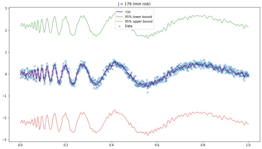
plt.figure(figsize=(14.5, 8))
r_hat, r_lower, r_upper, J_hat = estimate_r(X, Y, J=None)
plt.scatter(X, Y, color='C0', marker='x', alpha=0.5, label='Data')
plt.plot(X, r_hat(X), color='purple', label='$r(x)$')
plt.plot(X, r_lower(X), color='red', alpha=0.5, label='95% lower bound')
plt.plot(X, r_upper(X), color='green', alpha=0.5, label='95% upper bound')
plt.title('J = %i (min risk)' % J_hat)
plt.legend()
plt.show()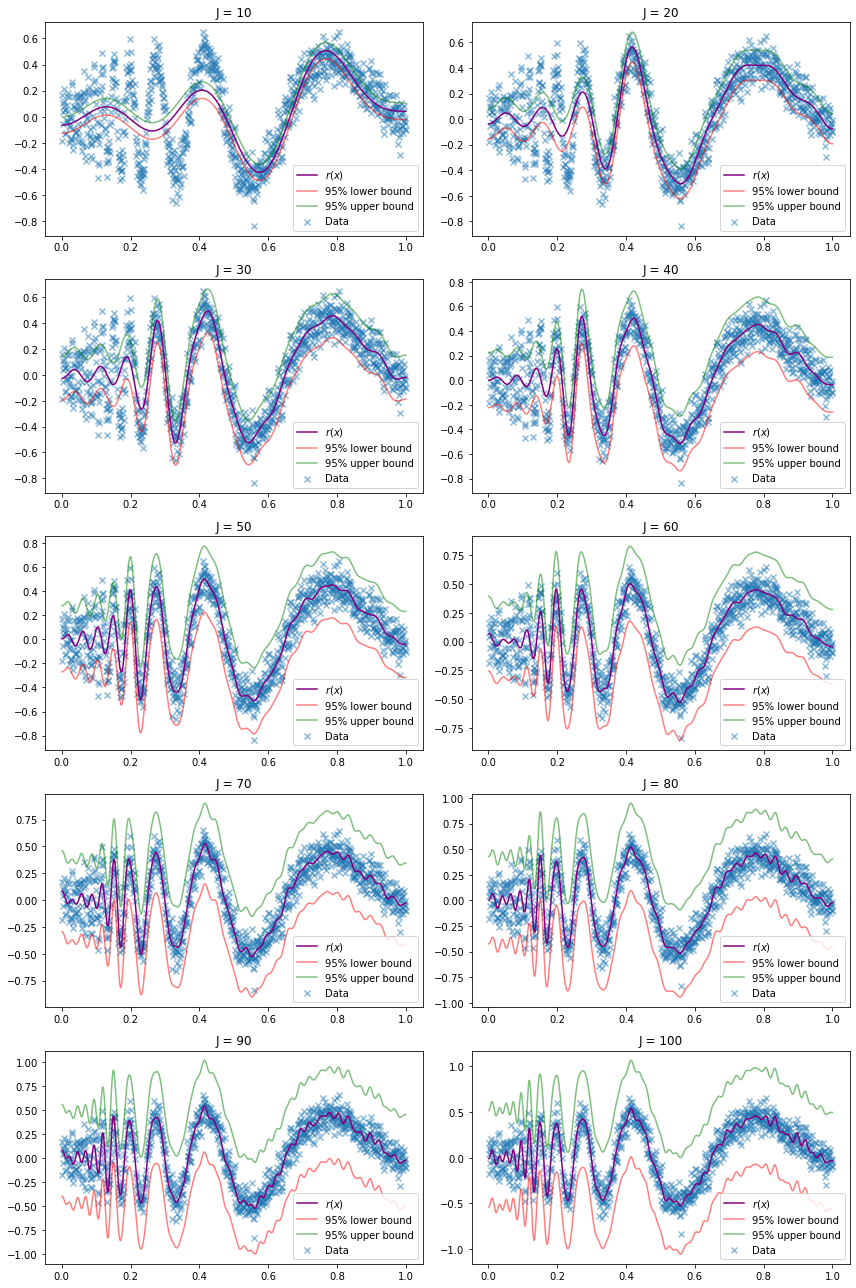
png
png
(b)
The father Haar wavelet of Haar scaling function is defined by
\[ \phi(x) = \begin{cases} 1 & \text{if } 0 \leq x < 1 \\ 0 & \text{otherwise} \end{cases} \]
The mother Haar wavelet is defined by
\[ \psi(x) = \begin{cases} -1 & \text{if } 0 \leq x \leq \frac{1}{2} \\ 1 & \text{if } \frac{1}{2} < x \leq 1 \end{cases} \]
For any integers \(j\) and \(k\) define
\[ \phi_{j, k}(x) = 2^{j/2} \phi(2^j x - k) \quad \text{and} \quad \psi_{j, k}(x) = 2^{j/2} \psi(2^j x - k) \]
The function \(\psi_{j, k}\) has the same shape as \(\psi\) but it has been rescaled by a factor of \(2^{j/2}\) and shifted by a factor of \(k\).
Let
\[ W_j = \{\psi_{j, k}, \; k = 0, 1, \dots, 2^j - 1\} \] where \[\psi_{j, k}(x) = 2^{j/2} \psi(2^j x - k)\]
be the set of rescaled and shifted mother wavelets at resolution \(j\).
Theorem 22.13. The set of functions
\[ \left\{ \phi, W_0, W_1, W_2, \dots \right\} \]
is an orthonormal basis for \(L_2(0, 1)\).
It follows from this theorem that we can expand any function \(f \in L_2(0, 1)\) in this basis. Because each \(W_j\) is itself a set of functions, we write the expansion as a double sum:
\[ f(x) = \alpha \phi(x) + \sum_{j=0}^\infty \sum_{k=0}^{2^j - 1} \beta_{j, k} \psi_{j, k}(x) \]
where
\[ \alpha = \int_0^1 f(x) \phi(x) dx, \quad \beta_{j, k} = \int_0^1 f(x) \psi_{j, k}(x) dx\]
We call \(\alpha\) the scaling coefficient and \(\beta_{j, k}\) the detail coefficients. We call the finite sum
\[ \tilde{f}(x) = \alpha \phi(x) + \sum_{j=0}^{J - 1} \sum_{k=0}^{2^j - 1} \beta_{j, k}\psi_{j, k}(x)\]
the resolution \(J\) approximation to \(f\). The total number of terms in this sum is
\[ 1 + \sum_{j=0}^{J - 1}2^j = 2^J\]
Haar wavelets are localized, meaning they are zero outside of an interval, but they are not smooth. In 1988, Ingrid Daubechie showed that such wavelets do exist. They can be constructed numerically, but there is no closed form formula for smoother wavelets. To keep things simple, we will continue to use Haar wavelets.
We can now use wavelets to do density estimation and regression. We shall only discuss the regression problem \(Y_i = r(x_i) + \sigma \epsilon_i\) where \(\epsilon_i \sim N(0, 1)\) and \(x_i = i / n\). To simplify this discussion we assume that \(n = 2^J\) for some \(J\).
There is one major difference between estimation using wavelets instead of a cosine (or polynomial) basis. With the cosine basis, we used all terms \(1 \leq j \leq J\) for some \(J\). With wavelets, we use a method called thresholding where we keep a term in the function approximation only if its coefficient is large. The simplest version is called hard, universal thresholding.
Haar Wavelet Regression
- Let \(J = \log_2 n\) and define
\[ \hat{\alpha} = \frac{1}{n} \sum_i \phi(x_i) Y_i \quad \text{and} \quad D_{j, k} = \frac{1}{n} \sum_i \psi_{j, k}(x_i) Y_i \]
for \(0 \leq j \leq J - 1\)
- Estimate \(\sigma\) by
\[ \hat{\sigma} = \sqrt{n} \; \times \; \frac{\text{median} \left( \left| D_{J-1, k} : k = 0, \dots, 2^{J - 1} - 1\right| \right)}{0.6745} \]
- Apply universal thresholding:
\[ \hat{\beta}_{j, k} = \begin{cases} D_{j, k} & \text{if } \left| D_{j, k} \right| > \hat{\sigma} \sqrt{\frac{2 \log n}{n}} \\ 0 & \text{otherwise} \end{cases}\]
- Set
\[ \hat{f}(x) = \hat{\alpha} \phi(x) + \sum_{j = j_0}^{J - 1} \sum_{k = 0}^{2^j - 1} \hat{\beta}_{j, k} \psi_{j, k}(x) \]
In practice, we do not compute \(\hat{\alpha}\) and \(D_{j, k}\). Instead, we use the discrete wavelet transform (DWT) which is very fast. For Haar wavelets, the DWT works as follows.
DWT for Haar Wavelets
- Let \(y = (Y_1, \dots, Y_n)\) and let \(J = \log_2 n\).
- Create a list \(D\) with elements \(D[0], ..., D[J - 1]\)
- Do:
temp <- y / sqrt(n)
for j in (J - 1):0 {
  m <- 2^j
  I <- (1:m)
  D[j] <- (temp[2 * I] - temp[(2 * I) - 1]) / sqrt(2)
  temp <- (temp[2 * I] + temp[(2 * I) - 1]) / sqrt(2)
}
# Wavelet base functions
import numpy as np
def haar_father_wavelet(x):
return np.where((x >= 0) & (x < 1), 1, 0)
def haar_mother_wavelet(x):
return np.where((x >= 0) & (x < 1), np.where(x <= 1/2, -1, 1), 0)
def psi_wavelet(j, k):
def f(x):
return 2**(j / 2) * haar_mother_wavelet((2**j)*x - k)
return fdef estimate_r(X, Y):
n = len(Y)
J = int(np.ceil(np.log2(n)))
def X_to_L2(t):
return (t - X.min()) / (X.max() - X.min())
xx = X_to_L2(X)
alpha_hat = np.sum(Y) / n
D = {}
for j in range(J):
D[j] = np.zeros(2**j)
for k in range(2**j):
D[j][k] = psi_wavelet(j, k)(xx) @ Y / n
sigma_hat = np.sqrt(n) * np.median(np.abs(D[J - 1])) / 0.6745
threshold = sigma_hat * np.sqrt(2 * np.log(n) / n)
beta_hat = [(j, k, v) for j, values in D.items() for k, v in enumerate(values) if np.abs(v) > threshold]
def r_hat(X):
xx = X_to_L2(X)
return alpha_hat * haar_father_wavelet(xx) \
+ np.sum(np.array([v * psi_wavelet(j, k)(xx) for j, k, v in beta_hat]), axis=0)
return r_hatr_hat = estimate_r(X, Y)import matplotlib.pyplot as plt
%matplotlib inline
plt.figure(figsize=(12, 8))
plt.scatter(X, Y, color='C0', alpha=0.5, marker='x', label='Data')
X_min, X_max = X.min(), X.max()
t = np.arange(X_min, X_max, step=(X_max - X_min) / 10000)
plt.plot(t, r_hat(t), color='purple', label='$\hat{r}(x)$')
plt.legend()
plt.show()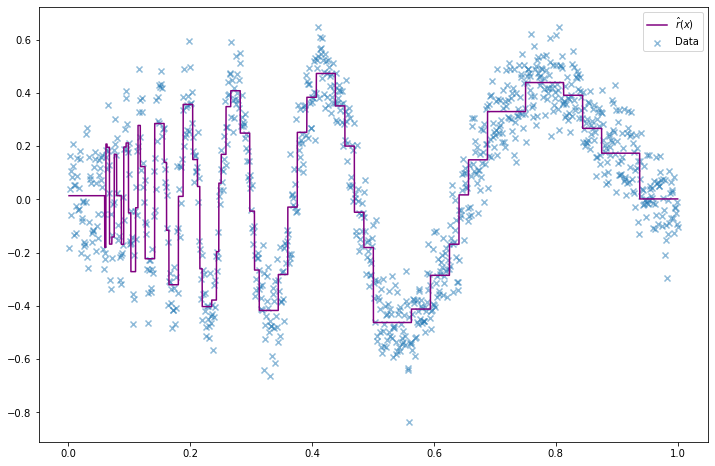
png
Exercise 22.6.10 (Haar density estimation). Let \(X_1, \dots, X_n \sim f\) for some density \(f\) on \([0, 1]\). Let’s consider constructing a wavelet histogram. Let \(\phi\) and \(\psi\) be the Haar father and mother wavelet. Write
\[ f(x) \approx \alpha\phi(x) + \sum_{j=0}^{J - 1} \sum_{k=0}^{2^j - 1} \beta_{j, k} \psi_{j, k}(x) \]
where \(J \approx \log_2(n)\) and
\[ \alpha = \int_0^1 f(x) \phi(x) dx, \quad \beta_{j, k} = \int_0^1 f(x) \psi_{j, k}(x) dx\] Let
\[ \hat{\beta}_{j, k} = \frac{1}{n} \sum_{i=1}^n \psi_{j, k}(X_i) \]
(a) Show that \(\hat{\beta}_{j, k}\) is an unbiased estimate of \(\beta_{j, k}\).
(b) Define the Haar histogram
\[ \hat{f}(x) = \phi(x) + \sum_{j=0}^{B} \sum_{k=0}^{2^j - 1} \hat{\beta}_{j, k} \psi_{j, k}(x) \]
for \(0 \leq B \leq J - 1\).
(c) Find an approximate expression for the MSE as a function of \(B\).
(d) Generate \(n = 1000\) observations from a \(\text{Beta}(15, 4)\) density. Estimate the density using the Haar histogram. Use leave-one-out cross validation to choose \(B\).
Solution.
(a)
\[ \mathbb{E}(\hat{\beta}_{j, k}) = \frac{1}{n} \sum_{i=1}^n \mathbb{E}(\psi_{j, k}(X_i)) = \mathbb{E}(\psi_{j, k}(X_1)) = \int_0^1 \psi_{j, k}(x) dx = \beta_{j, k} \]
(b) Let’s interpret “define” as “implement.”
# Wavelet base functions

import numpy as np

def haar_father_wavelet(x):
    return np.where((x >= 0) & (x < 1), 1, 0)

def haar_mother_wavelet(x):
    return np.where((x >= 0) & (x < 1),  np.where(x <= 1/2, -1, 1), 0)

def psi_wavelet(j, k):
    def f(x):
        return 2**(j / 2) * haar_mother_wavelet((2**j)*x - k)
return fimport numpy as np
def haar_histogram(X, B):
n = len(X)
def X_to_L2(t):
return (t - X.min()) / (X.max() - X.min())
xx = X_to_L2(X)
D = {}
for j in range(B):
D[j] = np.zeros(2**j)
for k in range(2**j):
D[j][k] = np.sum(psi_wavelet(j, k)(xx)) / n
# No thresholding
beta_hat = [(j, k, v) for j, values in D.items() for k, v in enumerate(values)]
def f_hat(x):
xx = X_to_L2(x)
return haar_father_wavelet(xx) \
+ np.sum(np.array([v * psi_wavelet(j, k)(xx) for j, k, v in beta_hat]), axis=0)
return f_hat(c) The orthonormal basis of Haar wavelets has its functions ordered as
\[ \begin{array}{ccc} \phi, \\ \psi_{0, 0}, \\ \psi_{1, 0}, & \psi_{1, 1}, \\ \psi_{2, 0}, & \dots, & \psi_{2, 2}, \\ \vdots \\ \psi_{j, 0}, & \dots, & \psi_{j, 2^k - 1}, \\ \vdots \end{array} \]
where each row of wavelets other than the first goes from \(\psi_{j, 0}\) to \(\psi_{j, 2^j - 1}\), containing \(2^j\) functions. We can label them in order
\[ q_1, q_2, \dots \quad \text{where }q_n = \begin{cases} \phi & \text{if } n = 1 \\ \psi_{\lceil \log_2 n \rceil- 1, n + 1 - \lceil \log_2 n \rceil } & \text{otherwise} \end{cases}\]
Now, limiting the Haar histogram estimator to hyperparameter \(B\) is equivalent to limiting it to only use the first \(2^{B + 1}\) functions.
Then, we can use Theorem 22.5 to calculate the risk on the basis of the \(q_j\)’s, where \(J = 2^{B + 1}\):
\[ R = \sum_{j=1}^J \frac{\sigma_j^2}{n} + \sum_{j=J+1}^\infty \beta_j^2 \]
with approximation
\[ \hat{R}_J(J) = \sum_{j=1}^J \frac{\hat{\sigma}_j^2}{n} + \sum_{j=J+1}^p \left( \hat{\beta}_j^2 - \frac{\hat{\sigma}_j^2}{n} \right)_{+} \]
where
\[ \hat{\sigma}_j^2 = \frac{1}{n - 1} \sum_{i=1}^n \left( q_j(X_i) - \hat{\beta}_j\right)^2 \]
Rewriting the approximation on the original Haar wavelet notation basis, we get:
\[ \hat{R}(B) = \frac{\hat{\sigma}_\phi^2}{n} + \sum_{j=0}^B \sum_{k=0}^{2^j - 1} \frac{\hat{\sigma}_{j, k}^2}{n} + \sum_{j=B+1}^p \sum_{k=0}^{2^j - 1} \left( \hat{\beta}_{j, k}^2 - \frac{\hat{\sigma}_{j, k}^2}{n} \right)_+ \]
where the estimated betas are still
\[ \hat{\beta}_{j, k} = \frac{1}{n} \sum_{i=1}^n \psi_{j, k} (X_i)\]
and the estimated variances are
\[ \hat{\sigma}_\phi^2 = \frac{1}{n - 1} \sum_{a=0}^B \sum_{b=0}^{2^a - 1} \left( \psi_{a, b}(X_i) - 1\right)^2 \quad \text{and} \quad \hat{\sigma}_{j, k}^2 = \frac{1}{n - 1} \sum_{a=0}^B \sum_{b=0}^{2^a - 1} \left( \psi_{a, b}(X_i) - \hat{\beta}_{j, k}\right)^2 \]
(d) Generate \(n = 1000\) observations from a \(\text{Beta}(15, 4)\) density. Estimate the density using the Haar histogram. Use leave-one-out cross validation to choose \(B\).
# Generate data
from scipy.stats import beta
X = beta.rvs(15, 4, size=1000)# Plot histograms for various B values
import matplotlib.pyplot as plt
%matplotlib inline
step = 1e-4
xx = np.arange(0, 1 + step, step)
import matplotlib.pyplot as plt
%matplotlib inline
def do_subplot(i, B):
ax = plt.subplot(5, 2, i)
f_hat = haar_histogram(X, B=B)
ax.plot(xx, f_hat(xx), color='purple')
ax.set_title('B = %i' % B)
plt.figure(figsize=(12, 12))
for i, J in enumerate([1, 2, 3, 4, 5, 6, 7, 8, 9, 10]):
do_subplot(i + 1, J)
plt.tight_layout()
plt.show()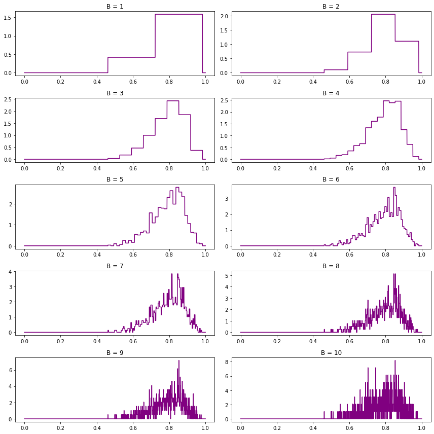
png
Rather than using the risk expression from (c), we will use the leave-one-out cross-validation score, as in definition 21.15:
\[ \hat{J} = \int \left( \hat{f}(x) \right)^2 dx - \frac{2}{n} \sum_{i=1}^n \hat{f}_{(-i)} (X_i) \]
where \(\hat{f}\) is the estimator using all data, and \(\hat{f}_{(-i)}\) is the estimator dropping the \(i\)-th observation.
def leave_one_out_risk_score(X, B):
estimator = lambda data: haar_histogram(data, B)
n = len(X)
f_hat = estimator(X)
step = 1e-4
X_min, X_max = X.min(), X.max()
xx = np.arange(X_min, X_max + step, step)
return (np.sum(f_hat(xx)**2) * step) \
- (2 / n) * np.sum([estimator(X[np.arange(n) != i])(X[i]) for i in range(n)])# Explicitly compute risk score for multiple B values
max_B = 8
risk_B = np.empty(max_B)
for B in range(1, max_B + 1):
risk_B[B - 1] = leave_one_out_risk_score(X, B)
selected_B = np.argmin(risk_B) + 1
selected_B_score = risk_B[selected_B - 1]# Plot risks and selected B value
plt.figure(figsize=(12, 8))
plt.plot(range(1, max_B + 1), risk_B)
plt.xlabel('B')
plt.ylabel(r'Risk score $\hat{J}$')
plt.show()
print('Selected B: %i' % selected_B)
print('Selected risk score: %.3f' % selected_B_score)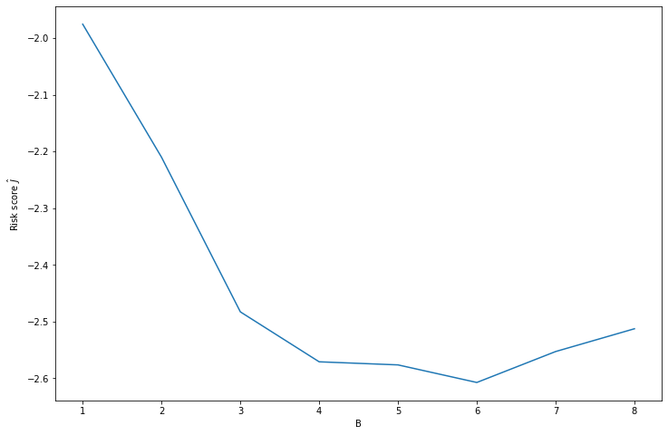
png
Selected B: 6
Selected risk score: -2.607f_hat = haar_histogram(X, B=selected_B)
plt.figure(figsize=(12, 8))
plt.plot(xx, f_hat(xx), color='purple')
plt.title('B = %i (min risk)' % selected_B)
plt.xlabel('X')
plt.ylabel(r'Risk score $\hat{J}$')
plt.show()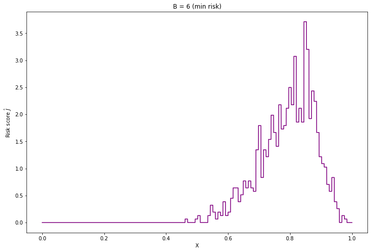
png
Exercise 22.6.11. In this exercise, we will explore the motivation for equation (22.38). Let \(X_1, \dots, X_n \sim N(0, \sigma^2)\). Let
\[ \hat{\sigma} = \sqrt{n} \times \frac{\text{median} (| X_1|, \dots, |X_n|)}{0.6745} \]
(a) Show that \(\mathbb{E}(\hat{\sigma}) = \sigma\).
(b) Simulate \(n = 100\) observations from a \(N(0, 1)\) distribution. Compute \(\hat{\sigma}\) as well as the usual estimate of \(\sigma\). Repeat 1000 times and compare the MSE.
(c) Repeat (b) but add some outliers to the data. To do this, simulate each observation from a \(N(0, 1)\) with probability .95 and simulate each observation from a \(N(0, 10)\) with probability 0.05.
Solution.
(a) This formula seems incorrect as is – there is no need to rescale by \(\sqrt{n}\).
From the Median Theorem, \(\mathbb{E}(\text{median}( \{ |X_i| : i = 1, \dots, n \} )) = \mathbb{E}(\text{median}(|X|))\), where \(X \sim N(0, \sigma^2)\). But the half normal distribution has CDF \(F(x) = \text{erf}\left(\frac{x}{\sigma \sqrt{2}}\right)\), so the median is \(F^{-1}\left(\frac{1}{2}\right) = \frac{\sigma \sqrt{2}}{\sqrt{\pi}} \approx 0.6745 \sigma\). Therefore, \(\mathbb{E}(\hat{\sigma}) = \sigma\).
(b) Simulate \(n = 100\) observations from a \(N(0, 1)\) distribution. Compute \(\hat{\sigma}\) as well as the usual estimate of \(\sigma\). Repeat 1000 times and compare the MSE.
import numpy as np
from scipy.stats import norm
def run_experiment(n=100, B=1000):
median_sigma_hat = np.empty(B)
sd_sigma_hat = np.empty(B)
for i in range(B):
X = norm.rvs(size=n)
median_sigma_hat[i] = np.median(np.abs(X)) / 0.6745
sd_sigma_hat[i] = X.std()
return median_sigma_hat, sd_sigma_hatmedian_sigma_hat, sd_sigma_hat = run_experiment(n=100, B=1000)print('E[Median sigma hat]:\t %.3f' % median_sigma_hat.mean())
print('E[SD sigma hat]: \t %.3f' % sd_sigma_hat.mean())
print('SE[Median sigma hat]:\t %.3f' % median_sigma_hat.std())
print('SE[SD sigma hat]:\t %.3f' % sd_sigma_hat.std())E[Median sigma hat]: 1.004
E[SD sigma hat]: 0.992
SE[Median sigma hat]: 0.115
SE[SD sigma hat]: 0.070As expected, both methodologies produce similar estimates for \(\sigma\), but the median estimate has a wider variance.
(c) Repeat (b) but add some outliers to the data. To do this, simulate each observation from a \(N(0, 1)\) with probability .95 and simulate each observation from a \(N(0, 10)\) with probability 0.05.
import numpy as np
from scipy.stats import norm
def run_experiment(n=100, B=1000):
median_sigma_hat = np.empty(B)
sd_sigma_hat = np.empty(B)
for i in range(B):
X1 = norm.rvs(size=n, scale=1)
X2 = norm.rvs(size=n, scale=10)
X = np.where(np.random.uniform(size=n) < 0.95, X1, X2)
median_sigma_hat[i] = np.median(np.abs(X)) / 0.6745
sd_sigma_hat[i] = X.std()
return median_sigma_hat, sd_sigma_hatmedian_sigma_hat, sd_sigma_hat = run_experiment(n=100, B=1000)print('E[Median sigma hat]:\t %.3f' % median_sigma_hat.mean())
print('E[SD sigma hat]: \t %.3f' % sd_sigma_hat.mean())
print('SE[Median sigma hat]:\t %.3f' % median_sigma_hat.std())
print('SE[SD sigma hat]:\t %.3f' % sd_sigma_hat.std())E[Median sigma hat]: 1.064
E[SD sigma hat]: 2.305
SE[Median sigma hat]: 0.124
SE[SD sigma hat]: 0.740The presence of 5% of outliers has significantly thrown off the usual estimate for \(\sigma\), while having a smaller effect on the median methodology.
Exercise 22.6.12. Repeat question 6 using the Haar basis.
Exercise 22.6.6
Expand the following functions in the cosine basis on \([0, 1]\). For (a) and (b), find the coefficients \(\beta_j\) analytically. For (c) and (d), find the coefficients \(\beta_j\) numerically, i.e.
\[ \beta_j = \int_0^1 f(x) \phi_j(x) \approx \frac{1}{N} \sum_{r=1}^N f \left( \frac{r}{N} \right) \phi_j \left( \frac{r}{N} \right) \]
for some large integer \(N\). Then plot the partial sum \(\sum_{j=1}^n \beta_j \phi_j(x)\) for increasing values of \(n\).
(a) \(f(x) = \sqrt{2} \cos (3 \pi x)\)
(b) \(f(x) = \sin(\pi x)\)
(c) \(f(x) = \sum_{j=1}^{11} h_j K(x - t_j)\), where \(K(t) = (1 + \text{sign}(t)) / 2\),
\[ (t_j) = (.1, .13, .15, .23, .25, .40, .44, .65, .76, .78, .81), \\ (h_j) = (4, -5, 3, -4, 5, -4.2, 2.1, 4.3, -3.1, 2.1, -4.2) \]
(d) \[f(x) = \sqrt{x(1-x)} \sin \left( \frac{2.1 \pi}{(x + .05)} \right) \]
Solution.
As in question 6, (a) and (b) are to be solved analytically, while (c) and (d) numerically. Plots are to be provided for all scenarios.
(a) \(f(x) = \sqrt{2} \cos (3 \pi x)\)
We have:
\[ \begin{align} \alpha &= \int_0^1 f(x) \phi(x) dx = \int_0^1 \sqrt{2} \cos (3 \pi x) dx = 0 \\ \beta_{j, k} &= \int_0^1 f(x) \psi_{j, k}(x) dx \\ &= 2^{(j + 1)/2} \left( \int_{\frac{k + 1/2}{2^j}}^{\frac{k + 1}{2^j}} \cos(3 \pi x) dx - \int_{\frac{k}{2^j}}^{\frac{k + 1/2}{2^j}} \cos(3 \pi x) dx \right) \\ &= \frac{2^{(j + 1)/2}}{3 \pi} \left( \sin\left( \frac{3\pi k}{2^j} \right) + \sin\left( \frac{3\pi (k + 1)}{2^j} \right) - 2 \sin\left( \frac{3\pi \left(k + \frac{1}{2}\right)}{2^j} \right) \right) \end{align} \]
# Wavelet base functions

import numpy as np

def haar_father_wavelet(x):
    return np.where((x >= 0) & (x < 1), 1, 0)

def haar_mother_wavelet(x):
    return np.where((x >= 0) & (x < 1),  np.where(x <= 1/2, -1, 1), 0)

def psi_wavelet(j, k):
    def f(x):
        return 2**(j / 2) * haar_mother_wavelet((2**j)*x - k)
return falpha = 0
def beta(j, k):
return (2**((j + 1)/2) / (3 * np.pi)) * \
(np.sin(3 * np.pi * k / 2**(j)) + np.sin(3 * np.pi * (k + 1) / 2**(j)) \
- (2 * np.sin(3 * np.pi * (k + 1/2) / 2**(j)) ))
def partial_sum(B, xx):
result = alpha * np.ones_like(xx)
for j in range(B+1):
for k in range(2**j):
result += beta(j, k) * psi_wavelet(j, k)(xx)
return result# Plot in separate boxes for ease of visualization
import matplotlib.pyplot as plt
%matplotlib inline
step = 1e-4
epsilon = 1e-12 # small shift to avoid spikes
xx = np.arange(0, 1, step) + epsilon
plt.figure(figsize=(12, 12))
def do_subplot(index, xx, yy, label, color):
ax = plt.subplot(4, 1, index)
ax.plot(xx, yy, label=label, color=color)
ax.legend()
do_subplot(1, xx, partial_sum(2, xx), label=r'$B = %i$' % 2, color='C0')
do_subplot(2, xx, partial_sum(4, xx), label=r'$B = %i$' % 4, color='C1')
do_subplot(3, xx, partial_sum(6, xx), label=r'$B = %i$' % 6, color='C2')
do_subplot(4, xx, np.sqrt(2) * np.cos(3 * np.pi * xx), label=r'$f(x) = \sqrt{2} \cos(3 \pi x)$', color='C3')
plt.tight_layout()
plt.legend()
plt.show()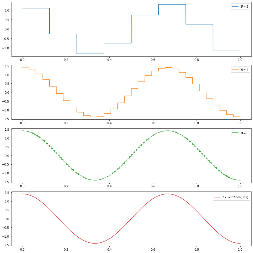
png
(b) \(f(x) = \sin(\pi x)\)
We have:
\[ \begin{align} \alpha &= \int_0^1 f(x) \phi(x) dx = \int_0^1 \sin (\pi x) dx = \frac{2}{\pi} \\ \beta_{j, k} &= \int_0^1 f(x) \psi_{j, k}(x) dx \\ &= 2^{j/2} \left( \int_{\frac{k + 1/2}{2^j}}^{\frac{k + 1}{2^j}} \sin(\pi x) dx - \int_{\frac{k}{2^j}}^{\frac{k + 1/2}{2^j}} \sin(\pi x) dx \right) \\ &= \frac{2^{j/2}}{\pi} \left( 2 \cos\left( \frac{\pi \left(k + \frac{1}{2}\right)}{2^j} \right) - \cos\left( \frac{\pi k}{2^j} \right) - \cos\left( \frac{\pi (k + 1)}{2^j} \right) \right) \end{align} \]
# Wavelet base functions

import numpy as np

def haar_father_wavelet(x):
    return np.where((x >= 0) & (x < 1), 1, 0)

def haar_mother_wavelet(x):
    return np.where((x >= 0) & (x < 1), np.where(x <= 1/2, -1, 1), 0)

def psi_wavelet(j, k):
    def f(x):
        return 2**(j / 2) * haar_mother_wavelet((2**j)*x - k)
    return f
alpha = 2 / np.pi
def beta(j, k):
return (2**(j/2) / np.pi) * \
(2 * np.cos(np.pi * (k + 1/2) / 2**(j)) \
- np.cos(np.pi * k / 2**(j)) - np.cos(np.pi * (k + 1) / 2**(j)))
def partial_sum(B, xx):
result = alpha * np.ones_like(xx)
for j in range(B+1):
for k in range(2**j):
result += beta(j, k) * psi_wavelet(j, k)(xx)
return result# Plot in separate boxes for ease of visualization
import matplotlib.pyplot as plt
%matplotlib inline
step = 1e-4
epsilon = 1e-12 # small shift to avoid spikes
xx = np.arange(0, 1, step) + epsilon
plt.figure(figsize=(12, 12))
def do_subplot(index, xx, yy, label, color):
ax = plt.subplot(4, 1, index)
ax.plot(xx, yy, label=label, color=color)
ax.legend()
do_subplot(1, xx, partial_sum(2, xx), label=r'$B = %i$' % 2, color='C0')
do_subplot(2, xx, partial_sum(4, xx), label=r'$B = %i$' % 4, color='C1')
do_subplot(3, xx, partial_sum(6, xx), label=r'$B = %i$' % 6, color='C2')
do_subplot(4, xx, np.sin(np.pi * xx), label=r'$f(x) = \sin(\pi x)$', color='C3')
plt.tight_layout()
plt.legend()
plt.show()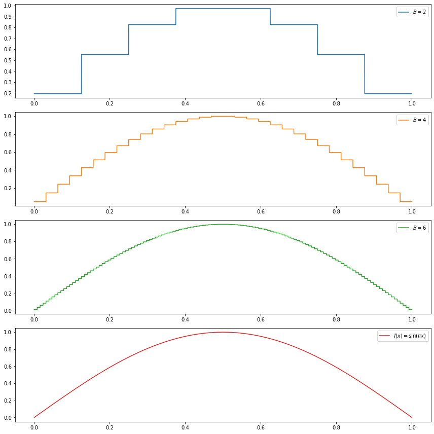
png
(c) \(f(x) = \sum_{j=1}^{11} h_j K(x - t_j)\), where \(K(t) = (1 + \text{sign}(t)) / 2\),
\[ (t_j) = (.1, .13, .15, .23, .25, .40, .44, .65, .76, .78, .81), \\ (h_j) = (4, -5, 3, -4, 5, -4.2, 2.1, 4.3, -3.1, 2.1, -4.2) \]
# Wavelet base functions

import numpy as np

def haar_father_wavelet(x):
    return np.where((x >= 0) & (x < 1), 1, 0)

def haar_mother_wavelet(x):
    return np.where((x >= 0) & (x < 1), np.where(x <= 1/2, -1, 1), 0)

def psi_wavelet(j, k):
    def f(x):
        return 2**(j / 2) * haar_mother_wavelet((2**j)*x - k)
return fimport numpy as np
T = np.array([.1, .13, .15, .23, .25, .40, .44, .65, .76, .78, .81])
H = np.array([4, -5, 3, -4, 5, -4.2, 2.1, 4.3, -3.1, 2.1, -4.2])
def f(x):
def K(t):
return (1 + np.sign(t))/2
return (H.reshape(1, -1) * K(
x.reshape(-1, 1).repeat(len(T), axis=1) - T.reshape(-1, 1).repeat(len(x), axis=1).T)
).sum(axis = 1)N = 10000
step = 1 / N
xx = np.arange(0, 1 + step, step=step)
alpha = f(xx) @ haar_father_wavelet(xx) / N
J = 256
estimated_beta = {}
for j in range(0, 7):
estimated_beta[j] = np.empty(2**j)
for k in range(2**j):
estimated_beta[j][k] = f(xx) @ psi_wavelet(j, k)(xx) / N
def beta(j, k):
return estimated_beta[j][k]def partial_sum(B, xx):
result = alpha * np.ones_like(xx)
for j in range(B+1):
for k in range(2**j):
result += beta(j, k) * psi_wavelet(j, k)(xx)
return result# Plot in separate boxes for ease of visualization
import matplotlib.pyplot as plt
%matplotlib inline
step = 1e-4
epsilon = 1e-12 # small shift to avoid spikes
xx = np.arange(0, 1, step) + epsilon
plt.figure(figsize=(12, 12))
def do_subplot(index, xx, yy, label, color):
ax = plt.subplot(4, 1, index)
ax.plot(xx, yy, label=label, color=color)
ax.legend()
do_subplot(1, xx, partial_sum(2, xx), label=r'$B = %i$' % 2, color='C0')
do_subplot(2, xx, partial_sum(4, xx), label=r'$B = %i$' % 4, color='C1')
do_subplot(3, xx, partial_sum(6, xx), label=r'$B = %i$' % 6, color='C2')
do_subplot(4, xx, f(xx), label=r'$f(x) = \sum_j h_j K(x - t_j) $', color='C3')
plt.tight_layout()
plt.legend()
plt.show()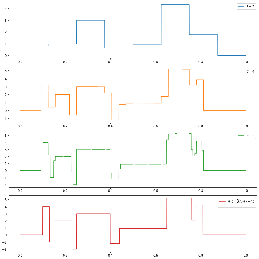
png
(d) $f(x) = ( ) $
# Wavelet base functions

import numpy as np

def haar_father_wavelet(x):
    return np.where((x >= 0) & (x < 1), 1, 0)

def haar_mother_wavelet(x):
    return np.where((x >= 0) & (x < 1), np.where(x <= 1/2, -1, 1), 0)

def psi_wavelet(j, k):
    def f(x):
        return 2**(j / 2) * haar_mother_wavelet((2**j)*x - k)
return fdef f(x):
return np.sqrt(x * (1 - x)) * np.sin(2.1 * np.pi / (x + 0.05))N = 10000
step = 1 / N
xx = np.arange(0, 1 + step, step=step)
alpha = f(xx) @ haar_father_wavelet(xx) / N
J = 256
estimated_beta = {}
for j in range(0, 7):
estimated_beta[j] = np.empty(2**j)
for k in range(2**j):
estimated_beta[j][k] = f(xx) @ psi_wavelet(j, k)(xx) / N
def beta(j, k):
return estimated_beta[j][k]def partial_sum(B, xx):
result = alpha * np.ones_like(xx)
for j in range(B+1):
for k in range(2**j):
result += beta(j, k) * psi_wavelet(j, k)(xx)
return result# Plot in separate boxes for ease of visualization
import matplotlib.pyplot as plt
%matplotlib inline
step = 1e-4
epsilon = 1e-12 # small shift to avoid spikes
xx = np.arange(0, 1, step) + epsilon
plt.figure(figsize=(12, 12))
def do_subplot(index, xx, yy, label, color):
ax = plt.subplot(4, 1, index)
ax.plot(xx, yy, label=label, color=color)
ax.legend()
do_subplot(1, xx, partial_sum(2, xx), label=r'$B = %i$' % 2, color='C0')
do_subplot(2, xx, partial_sum(4, xx), label=r'$B = %i$' % 4, color='C1')
do_subplot(3, xx, partial_sum(6, xx), label=r'$B = %i$' % 6, color='C2')
do_subplot(4, xx, f(xx), label=r'$f(x) = \sqrt{x (1 - x)} \sin \left( \frac{2.1 \pi}{(x + .05)} \right)$', color='C3')
plt.tight_layout()
plt.legend()
plt.show()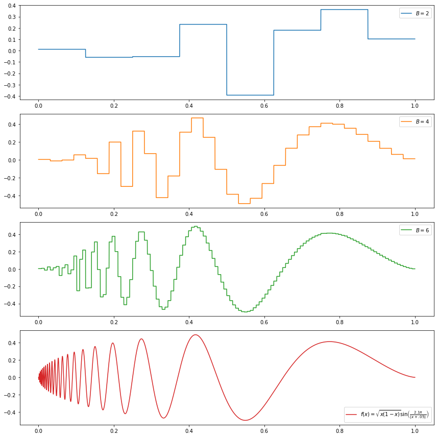
png