16. Inference about Independence
This chapter addresses two questions:
- How do we test if two random variables are independent?
- How do we estimate the strength of dependence between two random variables?
Recall we write \(Y \text{ ⫫ } Z\) to mean that \(Y\) and \(Z\) are independent.
When \(Y\) and \(Z\) are not independent, we say they are dependent or associated or related.
Note that dependence does not mean causation: - Smoking is related to heart disease, and quitting smoking will reduce the chance of heart disease. - Owning a TV is related to lower starvation, but giving a starving person a TV does not make them not hungry.
16.1 Two Binary Variables
Suppose that both \(Y\) and \(Z\) are binary. Consider a data set \((Y_1, Z_1), \dots, (Y_n, Z_n)\). Represent the data as a two-by-two table:
\[ \begin{array}{c|cc|c} & Y = 0 & Y = 1 & \\ \hline Z = 0 & X_{00} & X_{01} & X_{0\text{·}}\\ Z = 1 & X_{10} & X_{11} & X_{1\text{·}}\\ \hline & X_{\text{·}0} & X_{\text{·}1} & n = X_{\text{··}} \end{array} \]
where \(X_{ij}\) represents the number of observations where \((Z_k, Y_k) = (i, j)\). The dotted subscripts denote sums, e.g. \(X_{i\text{·}} = \sum_j X_{ij}\). Denote the corresponding probabilities by:
\[ \begin{array}{c|cc|c} & Y = 0 & Y = 1 & \\ \hline Z = 0 & p_{00} & p_{01} & p_{0\text{·}}\\ Z = 1 & p_{10} & p_{11} & p_{1\text{·}}\\ \hline & p_{\text{·}0} & p_{\text{·}1} & 1 \end{array} \]
where \(p_{ij} = \mathbb{P}(Z = i, Y = j)\). Let \(X = (X_{00}, X_{01}, X_{10}, X_{11})\) denote the vector of counts. Then \(X \sim \text{Multinomial}(n, p)\) where \(p = (p_{00}, p_{01}, p_{10}, p_{11})\).
The odds ratio is defined to be
\[ \psi = \frac{p_{00} p_{11}}{p_{01} p_{10}}\]
The log odds ratio is defined to be
\[ \gamma = \log \psi\]
Theorem 16.2. The following statements are equivalent:
- \(Y \text{ ⫫ } Z\)
- \(\psi = 1\)
- \(\gamma = 0\)
- For \(i, j \in \{ 0, 1 \}\), \(p_{ij} = p_{i\text{·}} p_{\text{·}j}\)
Now consider testing
\[ H_0: Y \text{ ⫫ } Z \quad \text{versus} \quad H_1: \text{not} (Y \text{ ⫫ } Z) \]
First consider the likelihood ratio test. Under \(H_1\), \(X \sim \text{Multinomial}(n, p)\) and the MLE is \(\hat{p} = X / n\). Under \(H_0\), again \(X \sim \text{Multinomial}(n, p)\) but \(p\) is subjected to the constraint \(p_{ij} = p_{i.} p_{.j}\). This leads to the following test.
Theorem 16.3 (Likelihood Ratio Test for Independence in a 2-by-2 table). Let
\[ T = 2 \sum_{i=0}^1 \sum_{j=0}^1 X_{ij} \log \left( \frac{X_{ij} X_{\text{··}}}{X_{i\text{·}} X_{\text{·}j}} \right)\]
Under \(H_0\), \(T \leadsto \chi_1^2\). Thus, an approximate level \(\alpha\) test is obtained by rejecting \(H_0\) when \(T > \chi_{1, \alpha}^2\).
Theorem 16.4 (Pearson’s \(\chi^2\) test for Independence in a 2-by-2 table). Let
\[ U = \sum_{i=0}^1 \sum_{j=0}^1 \frac{(X_{ij} - E_{ij})^2}{E_{ij}} \]
where
\[ E_{ij} = \frac{X_{i\text{·}} X_{\text{·}j}}{n}\]
Under \(H_0\), \(U \leadsto \chi_1^2\). Thus, an approximate level \(\alpha\) test is obtained by rejecting \(H_0\) when \(U > \chi_{1, \alpha}^2\).
Here’s the intuition for the Pearson test: Under \(H_0\), \(p_{ij} = p_{i\text{·}} p_{\text{·}j}\), so the MLE of \(p_{ij}\) is \(\hat{p}_{ij} = \hat{p}_{i\text{·}} \hat{p}_{\text{·}j} = \frac{X_{i\text{·}}}{n} \frac{X_{\text{·}j}}{n}\). Thus, the expected number of observations in the \((i, j)\) cell is \(E_{ij} = n \hat{p}_{ij} = \frac{X_{i\text{·}} X_{\text{·}j}}{n}\). The statistic \(U\) compares the observed and expected counts.
Theorem 16.6. The MLE’s of \(\psi\) and \(\gamma\) are
\[ \hat{\psi} = \frac{X_{00} X_{11}}{X_{01} X_{10}} , \quad \hat{\gamma} = \log \hat{\psi} \]
The asymptotic standard errors (computed from the delta method) are
\[ \begin{align} \hat{\text{se}}(\hat{\psi}) &= \sqrt{\frac{1}{X_{00}} + \frac{1}{X_{01}} + \frac{1}{X_{10}} + \frac{1}{X_{11}}}\\ \hat{\text{se}}(\hat{\gamma}) &= \hat{\psi} \hat{\text{se}}(\hat{\gamma}) \end{align} \]
Yet another test of independence is the Wald test for \(\gamma = 0\) given by \(W = (\hat{\gamma} - 0) / \hat{\text{se}}(\hat{\gamma})\).
A \(1 - \alpha\) confidence interval for \(\gamma\) is \(\hat{\gamma} \pm z_{\alpha/2} \hat{\text{se}}(\hat{\gamma})\).
A \(1 - \alpha\) confidence interval for \(\psi\) can be obtained in two ways. First, we could use \(\hat{\psi} \pm z_{\alpha/2} \hat{\text{se}}(\hat{\psi})\). Second, since \(\psi = e^{\gamma}\) we could use \(\exp \{\hat{\gamma} \pm z_{\alpha/2} \hat{\text{se}}(\hat{\gamma})\}\). This second method is usually more accurate.
16.2 Interpreting the Odds Ratios
Suppose event \(A\) has probability \(\mathbb{P}(A)\). The odds of \(A\) are defined as
\[\text{odds}(A) = \frac{\mathbb{P}(A)}{1 - \mathbb{P}(A)}\]
It follows that
\[\mathbb{P}(A) = \frac{\text{odds}(A)}{1 + \text{odds}(A)}\]
Let \(E\) be the event that someone is exposed to something (smoking, radiation, etc) and let \(D\) be the event that they get a disease. The odds of getting the disease given exposure are:
\[\text{odds}(D | E) = \frac{\mathbb{P}(D | E)}{1 - \mathbb{P}(D | E)}\]
and the odds of getting the disease given non-exposure are:
\[\text{odds}(D | E^c) = \frac{\mathbb{P}(D | E^c)}{1 - \mathbb{P}(D | E^c)}\]
The odds ratio is defined to be
\[\psi = \frac{\text{odds}(D | E)}{\text{odds}(D | E^c)}\]
If \(\psi = 1\) then the disease probability is the same for exposed and unexposed; this implies these events are independent. Recall that the log-odds ratio is defined as \(\gamma = \log \psi\). Independence corresponds to \(\gamma = 0\).
Consider this table of probabilities:
\[ \begin{array}{c|cc|c} & D^c & D & \\ \hline E^c & p_{00} & p_{01} & p_{0\text{·}}\\ E & p_{10} & p_{11} & p_{1\text{·}}\\ \hline & p_{\text{·}0} & p_{\text{·}1} & 1 \end{array} \]
Denote the data by
\[ \begin{array}{c|cc|c} & D^c & D & \\ \hline E^c & X_{00} & X_{01} & X_{0\text{·}}\\ E & X_{10} & X_{11} & X_{1\text{·}}\\ \hline & X_{\text{·}0} & X_{\text{·}1} & X_{\text{··}} \end{array} \]
Now
\[ \mathbb{P}(D | E) = \frac{p_{11}}{p_{10} + p_{11}} \quad \text{and} \quad \mathbb{P}(D | E^c) = \frac{p_{01}}{p_{00} + p_{01}} \]
and so
\[ \text{odds}(D | E) = \frac{p_{11}}{p_{10}} \quad \text{and} \quad \text{odds}(D | E^c) = \frac{p_{01}}{p_{00}} \]
and therefore
\[ \psi = \frac{p_{11}p_{00}}{p_{01}p_{10}}\]
To estimate the parameters, we have to consider how the data were collected. There are three methods.
Multinomial Sampling. We draw a sample from the population and, for each sample, record their exposure and disease status. In this case, \(X = (X_{00}, X_{01}, X_{10}, X_{11}) \sim \text{Multinomial}(n, p)\). We then estimates the probabilities in the table by \[\hat{p}_{ij} = X_{ij} / n\] and
\[ \hat{\psi} = \frac{\hat{p}_{11} \hat{p}_{00}}{\hat{p}_{01} \hat{p}_{10}} = \frac{X_{11} X_{00}}{X_{01} X_{10}}\]
Prospective Sampling (Cohort Sampling). We get some exposed and unexposed people and count the number with disease within each group. Thus,
\[ X_{01} \sim \text{Binomial}(X_{0\text{·}}, \mathbb{P}(D | E^c)) \quad \text{and} \quad X_{11} \sim \text{Binomial}(X_{1\text{·}}, \mathbb{P}(D | E)) \]
In this case we should write small letters \(x_{0\text{·}}, x_{1\text{·}}\) instead of capital letters $ X_{0}, X_{1}$ since they are fixed and not random, but we’ll keep using capital letters for notational simplicity.
We can estimate \(\mathbb{P}(D | E))\) and \(\mathbb{P}(D | E^c)\) but we cannot estimate all probabilities in the table. Still, we can estimate \(\psi\). Now:
\[\hat{\mathbb{P}}(D | E) = \frac{X_{11}}{X_{1\text{·}}} \quad \text{and} \quad \hat{\mathbb{P}}(D | E^c) = \frac{X_{01}}{X_{0\text{·}}} \]
Thus,
\[ \hat{\psi} = \frac{X_{11} X_{00}}{X_{01} X_{10}}\]
as before.
Case-Control (Retrospective Sampling). Here we get some diseased and non-diseased people and we observe how many are exposed. This is much more efficient if the disease is rare. Hence,
\[ X_{10} \sim \text{Binomial}(X_{\text{·}0}, \mathbb{P}(E | D^c)) \quad \text{and} \quad X_{11} \sim \text{Binomial}(X_{\text{·}1}, \mathbb{P}(E | D)) \]
From this data we can estimate \(\mathbb{P}(E | D)\) and \(\mathbb{P}(E | D^c)\). Surprisingly, we can still estimate \(\psi\). To understand why, note that
\[ \mathbb{P}(E | D) = \frac{p_{11}}{p_{01} + p_{11}}, \quad 1 - \mathbb{P}(E | D) = \frac{p_{01}}{p_{01} + p_{11}}, \quad \text{odds}(E | D) = \frac{p_{11}}{p_{01}} \]
By a similar argument,
\[\text{odds}(E | D^c) = \frac{p_{10}}{p_{00}}\]
Hence,
\[\frac{\text{odds}(E | D)}{\text{odds}(E | D^c)} = \frac{p_{11} p_{00}}{p_{01} p_{10}} = \psi\]
Therefore,
\[\hat{\psi} = \frac{X_{11} X_{00}}{X_{01} X_{10}}\]
In all three methods, the estimate of \(\psi\) turns out to be the same.
It is tempting to try to estimate \(\mathbb{P}(D | E) - \mathbb{P}(D | E^c)\). In a case-control design, this quantity is not estimable. To see this, we apply Bayes’ theorem to get
\[\mathbb{P}(D | E) - \mathbb{P}(D | E^c) = \frac{\mathbb{P}(E | D) \mathbb{P}(D))}{\mathbb{P}(E)} - \frac{\mathbb{P}(E^c | D) \mathbb{P}(D)}{\mathbb{P}(E^c)}\]
Because of the way we obtained the data, \(\mathbb{P}(D)\) is not estimable from the data.
However, we can estimate \(\xi = \mathbb{P}(D | E) / \mathbb{P}(D | E^c)\), which is called the relative risk, under the rare disease assumption.
Theorem 16.9. Let \(\xi = \mathbb{P}(D | E) / \mathbb{P}(D | E^c)\). Then
\[ \frac{\psi}{\xi} \rightarrow 1\]
as \(\mathbb{P}(D) \rightarrow 0\).
Thus, under the rare disease assumption, the relative risk is approximately the same as the odds ratio, which we can estimate.
In a randomized experiment, we can interpret a strong association, that is \(\psi \neq 1\), as a causal relationship. In an observational (non-randomized) study, the association can be due to other unobserved confounding variables. We’ll discuss causation in more detail later.
16.3 Two Discrete Variables
Now suppose that \(Y \in \{ 1, \dots, I \}\) and \(Z \in \{ 1, \dots, J \}\) are two discrete variables. The data can be represented by an \(I \times J\) table of contents:
\[ \begin{array}{c|cccccc|c} & Y = 1 & Y = 2 & \cdots & Y = j & \cdots & Y = J & \\ \hline Z = 1 & X_{11} & X_{12} & \cdots & X_{1j} & \cdots & X_{1J} & X_{1\text{·}}\\ Z = 2 & X_{21} & X_{22} & \cdots & X_{2j} & \cdots & X_{2J} & X_{2\text{·}}\\ \vdots & \vdots & \vdots & \vdots & \vdots & \vdots & \vdots & \vdots\\ Z = i & X_{i1} & X_{i2} & \cdots & X_{ij} & \cdots & X_{iJ} & X_{i\text{·}}\\ \vdots & \vdots & \vdots & \vdots & \vdots & \vdots & \vdots & \vdots\\ Z = I & X_{I1} & X_{I2} & \cdots & X_{Ij} & \cdots & X_{IJ} & X_{I\text{·}}\\ \hline & X_{\text{·}1} & X_{\text{·}1} & \cdots & X_{\text{·}j} & \cdots & X_{\text{·}J} & n \end{array} \]
Consider testing
\[ H_0: Y \text{ ⫫ } Z \quad \text{versus} \quad H_1: \text{not } H_0 \]
Theorem 16.10. Let
\[ T = 2 \sum_{i=1}^I \sum_{j=1}^J X_{ij} \log \left( \frac{X_{ij} X_{\text{··}}}{X_{i\text{·}} X_{\text{·}j}} \right) \]
The limiting distribution of \(T\) under the null hypothesis of independence is \(\chi^2_\nu\) where \(\nu = (I - 1)(J - 1)\).
Pearson’s \(\chi^2\) test statistic is
\[ U = \sum_{i=1}^I \sum_{j=1}^J \frac{(n_{ij} - E_{ij})^2}{E_{ij}}\]
Asymptotically, under \(H_0\), \(U\) has a \(\chi^2_\nu\) distribution where \(\nu = (I - 1)(J - 1)\).
There are a variety of ways to quantify the strength of dependence between two discrete variables \(Y\) and \(Z\). Most of them are not very intuitive. The one we shall use is not standard but is more interpretable.
We define
\[\delta(Y, Z) = \max_{A, B} \Big|\; \mathbb{P}_{Y, Z}(Y \in A, Z \in B) - \mathbb{P}_Y(Y \in A)\mathbb{P}_Z(Z \in B) \;\Big|\]
where the maximum is over all pairs of events \(A\) and \(B\).
Note: the original version on the book contains a typo; it is originally stated as
\[\delta(Y, Z) = \max_{A, B} \Big|\; \mathbb{P}_{Y, Z}(Y \in A, Z \in B) - \mathbb{P}_Y(Y \in A) - \mathbb{P}_Z(Z \in B) \;\Big|\]
For more context, this is a specific case of the “total variation distance” \(\delta(P_1, P_2)\) between the probability metrics \(P_1(Y, Z) = \mathbb{P}_{Y, Z}(Y \in A, Z \in B)\) and \(P_2(Y, Z) = \mathbb{P}_Y(Y \in A)\mathbb{P}_Z(Z \in B)\).
Theorem 16.12. Properties of \(\delta(Y, Z)\):
- \(0 \leq \delta(Y, Z) \leq 1\)
- \(\delta(Y, Z) = 0\) if and only if \(Y \text{ ⫫ } Z\)
- The following identity holds:
\[ \delta(X, Y) = \frac{1}{2} \sum_{i=1}^I \sum_{j=1}^J \Big|\; p_{ij} - p_{i\text{·}} p_{\text{·}j} \;\Big|\]
- The MLE of \(\delta\) is
\[ \hat{\delta}(X, Y) = \frac{1}{2} \sum_{i=1}^I \sum_{j=1}^J \Big|\; \hat{p}_{ij} - \hat{p}_{i\text{·}} \hat{p}_{\text{·}j} \;\Big|\]
where
\[ \hat{p}_{ij} = \frac{X_{ij}}{n}, \quad \hat{p}_{i\text{·}} = \frac{X_{i\text{·}}}{n}, \quad \hat{p}_{\text{·}j} = \frac{X_{\text{·}j}}{n} \]
The interpretation of \(\delta\) is this: if one person makes probability statements assuming independence and another person makes probability statements without assuming independence, their probability statements may differ by as much as \(\delta\). Here’s a suggested scale for interpreting \(\delta\):
| range | interpretation |
|---|---|
| 0 to 0.01 | negligible association |
| 0.01 to 0.05 | non-negligible association |
| 0.05 to 0.1 | substantial association |
| over 0.1 | very strong association |
A confidence interval for \(\delta\) can be obtained by bootstrapping. The steps are:
- Draw \(X^* \sim \text{Multinomial}(n, \hat{p})\);
- Compute \(\hat{p}_ij, \hat{p}_{i\text{·}}, \hat{p}_{\text{·}j}\);
- Compute \(\delta^*\);
- Repeat.
Now we use any of the methods we learned earlier for constructing bootstrap confidence intervals. However, we should not use a Wald interval in this case. The reason is that if \(Y\) and \(Z\) are independent then \(\delta = 0\) and we are on the boundary of the parameter space. In this case, the Wald method is not valid.
16.4 Two Continuous Variables
Now suppose that \(Y\) and \(Z\) are both continuous. If we assume that the joint distribution of \(Y\) and \(Z\) is bivariate Normal, then we measure the dependence between \(Y\) and \(Z\) by means of the correlation coefficient \(\rho\). Tests, estimates, and confidence intervals for \(\rho\) in the Normal case are given in the previous chapter. If we do not assume normality, then we need a nonparametric method for asserting dependence.
Recall that the correlation is
\[\rho = \frac{\mathbb{E}((X_1 - \mu_1)(X_2 - \mu_2))}{\sigma_1 \sigma_2} \]
A nonparametric estimator of \(\rho\) is the plug-in estimator which is:
\[\hat{\rho} = \frac{\sum_{i=1}^n (X_{1i} - \overline{X}_1)(X_{2i} - \overline{X}_2)}{\sqrt{\sum_{i=1}^n (X_{1i} - \overline{X}_1)^2 \sum_{i=1}^n (X_{2i} - \overline{X}_2)^2}} \]
which is just the sample correlation. A confidence interval can be constructed using the bootstrap. A test for \(\rho = 0\) can be based on the Wald test using the bootstrap to estimate the standard error.
The plug-in approach is useful for large samples. For small samples, we measure the correlation using the Spearman rank correlation coefficient \(\hat{\rho}_S\). We simply replace the data by their ranks, ranking each variable separately, then compute the correlation coefficient of the ranks.
To test the null hypothesis that \(\rho_S = 0\), we need the distribution of \(\hat{\rho}_S\) under the null hypothesis. This can be obtained by simulation. We fix the ranks of the first variable as \(1, 2, \dots, n\). The ranks of the second variable are chosen at random from the set of \(n!\) possible orderings, then we compute the correlation. This is repeated many times, and the resulting distribution \(\mathbb{P}_0\) is the null distribution of \(\hat{\rho}_S\). The p-value for the test is \(\mathbb{P}_0(|R| > |\hat{\rho}_S|)\) where \(R\) is drawn from the null distribution \(\mathbb{P}_0\).
16.5 One Continuous Variable and One Discrete
Suppose that \(Y \in \{ 1, \dots, I \}\) is discrete and \(Z\) is continuous. Let \(F_i(z) = \mathbb{P}(Z \leq z | Y = i)\) denote the CDF of \(Z\) conditional on \(Y = i\).
Theorem 16.15. When \(Y \in \{ 1, 2, \dots, I \}\) is discrete and \(Z\) is continuous, then \(Y \text{ ⫫ } Z\) if and only if \(F_1 = F_2 = \dots = F_I\).
It follows that to test for independence, we need to test
\[ H_0: F_1 = \dots = F_I \quad \text{versus} \quad H_1: \text{not } H_0 \]
For simplicity, we consider the case where \(I = 2\). To test the null hypothesis that \(F_1 = F_2\) we will use the two sample Kolmogorov-Smirnov test.
Let \(n_k\) denote the number of observations for which \(Y_i = k\). Let
\[\hat{F}_k(z) = \frac{1}{n_k} \sum_{i=1}^n I(Z_i \leq z) I(Y_i = k)\]
denote the empirical distribution function of \(Z\) given \(Y = k\). Define the test statistic
\[ D = \sup_x | \hat{F}_1(x) - \hat{F}_2(x) |\]
Theorem 16.16. Let
\[ H(t) = 1 - 2 \sum_{j=1}^\infty (-1)^{j-1} e^{-2j^2t^2} \]
Under the null hypothesis that \(F_1 = F_2\),
\[ \lim_{n \rightarrow \infty} \mathbb{P} \left( \sqrt{\frac{n_1 n_2}{n_1 + n_2}} D \leq t \right) = H(t) \]
It follows from the theorem than an approximate level \(\alpha\) test is obtained by rejecting \(H_0\) when
\[ \sqrt{\frac{n_1 n_2}{n_1 + n_2}} D > H^{-1}(1 - \alpha) \]
16.7 Exercises
Exercise 16.7.1. Prove Theorem 16.2.
The following statements are equivalent:
- \(Y \text{ ⫫ } Z\)
- \(\psi = 1\)
- \(\gamma = 0\)
- For \(i, j \in \{ 0, 1 \}\), \(p_{ij} = p_{i\text{·}} p_{\text{·}j}\)
Solution.
\(Y\) and \(Z\) are independent if and only if \(\mathbb{P}(Y = j | Z = i) = \mathbb{P}(Y = j) \mathbb{P}(Z = i)\) for all \(i\) and \(j\), so (1) and (4) are equivalent.
\(\gamma = \log \psi\), so (2) and (3) are equivalent.
Finally, \[ \begin{array}{c|cc|c} & Y = 0 & Y = 1 & \\ \hline Z = 0 & p_{00} & p_{01} & p_{0\text{·}}\\ Z = 1 & p_{10} & p_{11} & p_{1\text{·}}\\ \hline & p_{\text{·}0} & p_{\text{·}1} & 1 \end{array} \] The odds ratio is defined to be
\[ \psi = \frac{p_{00} p_{11}}{p_{01} p_{10}}\]
The log odds ratio is defined to be
\[ \gamma = \log \psi\]
\[ \begin{align} &\psi = 1\\ &\Leftrightarrow \frac{\text{odds}(Y | Z = 1)}{\text{odds}(Y | Z = 0)} = 1 \\ &\Leftrightarrow \text{odds}(Y | Z = 1) = \text{odds}(Y | Z = 0) \\ &\Leftrightarrow \mathbb{P}(Y | Z = 1) = \mathbb{P}(Y | Z = 0) \\ &\Leftrightarrow Y \text{ ⫫ } Z \end{align} \]
so (1) and (2) are equivalent.
Therefore, all statements are equivalent.
Exercise 16.7.2. Prove Theorem 16.3.
Let
\[ T = 2 \sum_{i=0}^1 \sum_{j=0}^1 X_{ij} \log \left( \frac{X_{ij} X_{\text{··}}}{X_{i\text{·}} X_{\text{·}j}} \right)\]
Under \(H_0\), \(T \leadsto \chi_1^2\). Thus, an approximate level \(\alpha\) test is obtained by rejecting \(H_0\) when \(T > \chi_{1, \alpha}^2\).
Solution. Let \(E_{ij} = \frac{X_{i\text{·}} X_{\text{·}j}}{X_\text{··}}\). We can rewrite the test statistic as
\[ T = 2 \sum_{i, j} X_{ij} \log \frac{X_{ij}}{E_{ij}} \]
The interpretation of \(E_{ij}\) is that it is the expected count in cell \((i, j)\) under \(H_0\):
\[ \begin{align} \mathbb{E}_{H_0}(Y = i, Z = j) &= n \mathbb{P}_{H_0}(Y = i, Z = j) \\ &= n \mathbb{P}(Y = i) \mathbb{P}(Z = j) \\ &= n \hat{p}_{i\text{·}} \hat{p}_{\text{·}j} \\ &= X_{\text{··}} \frac{X_{i\text{·}}}{X_{\text{··}}} \frac{X_{\text{·}j}}{X_{\text{··}}} \\ &= E_{ij} \end{align} \]
Now, the result will follow by applying the log-likelihood test between \(H_0\) and \(H_1\). The test statistic is:
\[ 2 \log \frac{\mathcal{L}(\tilde{p} | X)}{\mathcal{L}(\hat{p} | X)} = 2 \log \frac{\prod_{i, j} \tilde{p}_{ij}^{X_{ij}}}{\prod_{i, j} \hat{p}_{ij}^{X_{ij}}}\]
where \(\tilde{p}\) is the MLE under \(H_1\) and \(\hat{p}\) is the MLE under \(H_0\). But we have:
\[ \tilde{p}_{ij} = \frac{X_{ij}}{n} \quad \text{and} \quad \hat{p}_{ij} = \frac{E_{ij}}{n} \]
Substituting the MLEs on the log-likelihood ratio, we get
\[ 2 \log \frac{\mathcal{L}(\tilde{p} | X)}{\mathcal{L}(\hat{p} | X)} = 2 \log \prod_{i, j} \left( \frac{X_{ij}}{E_{ij}} \right)^{X_{ij}} = 2 \sum_{i, j} X_{ij} \log \frac{X_{ij}}{E_{ij}} \]
which is the desired result.
Reference: “G-test.” Wikipedia: The Free Encyclopedia. Wikimedia Foundation, Inc. 22 July 2004. Web. 17 Mar. 2020, en.wikipedia.org/w/index.php?title=G-test&oldid=914538756
Exercise 16.7.3. Prove Theorem 16.9.
Let \(\xi = \mathbb{P}(D | E) / \mathbb{P}(D | E^c)\). Then
\[ \frac{\psi}{\xi} \rightarrow 1\]
as \(\mathbb{P}(D) \rightarrow 0\).
Solution.
Consider this table of probabilities:
\[ \begin{array}{c|cc|c} & D^c & D & \\ \hline E^c & p_{00} & p_{01} & p_{0\text{·}}\\ E & p_{10} & p_{11} & p_{1\text{·}}\\ \hline & p_{\text{·}0} & p_{\text{·}1} & 1 \end{array} \]
Denote the data by
\[ \begin{array}{c|cc|c} & D^c & D & \\ \hline E^c & X_{00} & X_{01} & X_{0\text{·}}\\ E & X_{10} & X_{11} & X_{1\text{·}}\\ \hline & X_{\text{·}0} & X_{\text{·}1} & X_{\text{··}} \end{array} \]
Now
\[ \mathbb{P}(D | E) = \frac{p_{11}}{p_{10} + p_{11}} \quad \text{and} \quad \mathbb{P}(D | E^c) = \frac{p_{01}}{p_{00} + p_{01}} \]
and so
\[ \text{odds}(D | E) = \frac{p_{11}}{p_{10}} \quad \text{and} \quad \text{odds}(D | E^c) = \frac{p_{01}}{p_{00}} \]
and so
\[ \xi = \frac{\mathbb{P}(D | E)}{\mathbb{P}(D | E^c)} = \frac{p_{11} (p_{00} + p_{01})}{p_{01} (p_{10} + p_{11})} \]
Since
\[ \psi = \frac{p_{11}p_{00}}{p_{01}p_{10}}\]
we have:
\[ \frac{\psi}{\xi} = \frac{p_{11}p_{00}}{p_{01}p_{10}} \frac{p_{01} (p_{10} + p_{11})}{p_{11} (p_{00} + p_{01})} = \frac{p_{00}}{p_{10}} \frac{p_{1\text{·}}}{p_{0\text{·}}} \]
As \(\mathbb{P}(D) = p_{01} + p_{11} \rightarrow 0\) and the probabilites are non-negative, \(p_{01} \rightarrow 0\), \(p_{11} \rightarrow 0\), so
\[ \frac{\psi}{\xi} \rightarrow \frac{p_{00}}{p_{10}} \frac{p_{10}}{p_{00}} = 1 \]
Exercise 16.7.4. Prove equation (16.14).
\[ \delta(X, Y) = \max_{A, B} \Big|\; \mathbb{P}_{X, Y}(X \in A, Y \in B) - \mathbb{P}_X(X \in A) \mathbb{P}_Y(Y \in B) \;\Big| \]
is equivalent to
\[ \delta(X, Y) = \frac{1}{2} \sum_{i=1}^I \sum_{j=1}^J \Big|\; p_{ij} - p_{i\text{·}} p_{\text{·}j} \;\Big|\]
Solution.
As noted when the definition was introduced, this definition of \(\delta(X, Y)\) is a particular case of the total variation distance between metrics \(P_1(X, Y) = \mathbb{P}_{X, Y}(X \in A, Y \in B)\) and \(P_2(X, Y) = \mathbb{P}_X(X \in A) \mathbb{P}_Y(Y \in B)\), where
\[ \delta(P, Q) = \sup_{A \in \mathcal{F}} |P(A) - Q(A)| \]
and \(P, Q\) are two probability measures on a sigma-algebra \(\mathcal{F}\) of subsets from the sample space \(\Omega\).
(Note that \(P_1(X = i, Y = j) = p_{ij}\) and \(P_2(X = i, Y = j) = p_{i\text{·}} p_{\text{·}j}\)).
It is a known property of the total variation distance in countable spaces that
\[ \delta(P, Q) = \max_{A \in \mathcal{F}} |P(A) - Q(A)| = \frac{1}{2} \Vert P - Q \Vert_1 = \frac{1}{2} \sum_{\omega \in \Omega} \vert P(\omega) - Q(\omega) \vert\]
Let’s demonstrate it, following the steps in the reference below.
Let \(\mathcal{F}^+ \subset \mathcal{F}\) be the set of states \(\omega\) such that \(P(\omega) \geq Q(\omega)\), and let \(\mathcal{F}^- = \mathcal{F} - S^+\) be the set of states \(\omega\) such that \(P(\omega) < Q(\omega)\). We have:
\[ \max_{A \in \mathcal{F}} P(A) - Q(A) = P(\mathcal{F}^+) - Q(\mathcal{F}^+)\]
and
\[ \max_{A \in \mathcal{F}} Q(A) - P(A) = Q(\mathcal{F}^-) - P(\mathcal{F}^-)\]
But since \(P(\Omega) = Q(\Omega) = 1\), we have
\[ P(\mathcal{F}^+) + P(\mathcal{F}^-) = Q(\mathcal{F}^+) + Q(\mathcal{F}^-) = 1 \]
which implies that
\[ P(\mathcal{F}^+) - Q(\mathcal{F}^+) = Q(\mathcal{F}^-) - P(\mathcal{F}^-)\]
hence
\[ \max_{A \in \mathcal{F}} P(A) - Q(A) = \vert P(\mathcal{F}^+) - Q(\mathcal{F}^+) \vert = \vert Q(\mathcal{F}^-) - P(\mathcal{F}^-) \vert \]
Finally, since
\[ \vert P(\mathcal{F}^+) - Q(\mathcal{F}^+) \vert + \vert Q(\mathcal{F}^-) - P(\mathcal{F}^-) \vert = \sum_{\omega \in \Omega} | P(\omega) - Q(\omega) | = \Vert P - Q \Vert_1 \]
we have that
\[ \max_{A \in \mathcal{F}} |P(A) - Q(A)| = \frac{1}{2} \Vert P - Q \Vert_1 \]
which completes the proof.
Reference: Upfal, E., and M. Mitzenmacher. “Probability and computing.” (2005). Lemma 11.1, pg. 272-273.
Exercise 16.7.5. The New York Times (January 8, 2003, page A12) reported the following data on death sentencing and rance, from a study in Maryland:
| Death Sentence | No Death Sentence | |
|---|---|---|
| Black Victim | 14 | 641 |
| White Victim | 62 | 594 |
Analyse the data using the tools from this Chapter. Interpret the results. Explain why, based only on this information, you can’t make causal conclusions. (The authors of the study did use much more information in their full report).
Solution.
The statistic for the log-likelihood test for independence is is:
\[ T = 2 \sum_{i, j} X_{ij} \log \frac{X_{ij} X_{\text{··}}}{X_{i\text{·}} X_{\text{·}j}} \]
The statistic for Pearson’s \(\chi^2\) test is:
\[ U = \sum_{i, j} \frac{(X_{ij} - E_{ij})^2}{E_{ij}}\]
import numpy as np

X_ij = np.array([[14, 641], [62, 594]])
X_idot = X_ij.sum(axis = 1).reshape(2, 1)
X_dotj = X_ij.sum(axis = 0).reshape(1, 2)
n = X_ij.sum()
E_ij = X_idot @ X_dotj / n
# Log-likelihood test statistic
T = 2 * (X_ij * np.log(X_ij / E_ij)).sum()
# Pearson's \chi^2 test statistic
U = ((X_ij - E_ij)**2 / E_ij).sum()X_idotarray([[655],
[656]])X_dotjarray([[ 76, 1235]])E_ijarray([[ 37.97101449, 617.02898551],
[ 38.02898551, 617.97101449]])from scipy.stats import chi2
p_value_log_likelihood = 1 - chi2.cdf(T, 1)
p_value_pearson = 1 - chi2.cdf(U, 1)
print('T test statistic: \t\t%.3f'% T)
print('Pearson chi^2 statistic: \t%.3f'% U)
print('p-value log likelihood:\t\t %.3f' % p_value_log_likelihood)
print('p-value Pearson: \t\t %.3f' % p_value_pearson)T test statistic: 34.534
Pearson chi^2 statistic: 32.104
p-value log likelihood: 0.000
p-value Pearson: 0.000Both tests indicate that these variables are correlated. Note that this is not sufficient information, in itself, to imply causation.
from itertools import product

p = X_ij / n
p_idot = X_idot / n
p_dotj = X_dotj / n

delta = sum([abs(p[i, j] - p_idot[i, :] * p_dotj[:, j]) for (i, j) in product(range(2), range(2))]) / 2

print('delta(X, Y): %.3f' % delta)
delta(X, Y): 0.037\(\delta(X, Y)\) is between 0.01 and 0.05, suggesting a non-negligible association.
for (i, j) in product(range(2), range(2)):
    print(i,j)
0 0
0 1
1 0
1 1p_idotarray([[0.49961861],
[0.50038139]])p_idot[0, :]array([0.49961861])p_dotjarray([[0.05797101, 0.94202899]])p_idot[0, :] * p_dotj[:, 1]array([0.47065521])Exercise 16.7.6. Analyse the data on the variables Age and Financial Status from:
http://lib.stat.cmu.edu/DASL/Datafiles/montanadat.html
Solution.
import pandas as pd

data = pd.read_csv('data/montana.csv')

# Select wanted columns and remove missing data
data = data[['AGE', 'FIN']].replace('*', np.nan).dropna().astype(int)
data| AGE | FIN | |
|---|---|---|
| 0 | 3 | 2 |
| 1 | 2 | 3 |
| 2 | 1 | 2 |
| 3 | 3 | 1 |
| 4 | 3 | 2 |
| … | … | … |
| 203 | 1 | 3 |
| 205 | 1 | 3 |
| 206 | 3 | 2 |
| 207 | 3 | 1 |
| 208 | 2 | 2 |
207 rows × 2 columns
# Count occurrences in each cell
X_ij = np.zeros((3, 3)).astype(int)

for index, row in data.iterrows():
     X_ij[row['AGE'] - 1, row['FIN'] - 1] += 1

X_ij
array([[21, 16, 34],
[17, 23, 26],
[22, 37, 11]])X_idot = X_ij.sum(axis = 1).reshape(3, 1)
X_dotj = X_ij.sum(axis = 0).reshape(1, 3)
n = X_ij.sum()
E_ij = X_idot @ X_dotj / n
# Log-likelihood test statistic
T = 2 * (X_ij * np.log(X_ij / E_ij)).sum()
# Pearson's \chi^2 test statistic
U = ((X_ij - E_ij)**2 / E_ij).sum()from scipy.stats import chi2
p_value_log_likelihood = 1 - chi2.cdf(T, 4)
p_value_pearson = 1 - chi2.cdf(U, 4)
print('T test statistic: \t\t%.3f'% T)
print('Pearson chi^2 statistic: \t%.3f'% U)
print('p-value log likelihood:\t\t %.3f' % p_value_log_likelihood)
print('p-value Pearson: \t\t %.3f' % p_value_pearson)T test statistic: 22.064
Pearson chi^2 statistic: 20.679
p-value log likelihood: 0.000
p-value Pearson: 0.000Both tests indicate correlation between the two sequences.
from itertools import product

p = X_ij / n
p_idot = X_idot / n
p_dotj = X_dotj / n

delta = sum([abs(p[i, j] - p_idot[i, :] * p_dotj[:, j]) for (i, j) in product(range(3), range(3))]) / 2

print('delta(X, Y): %.3f' % delta)
delta(X, Y): 0.128\(\delta(X, Y) > 0.1\) indicates a strong correlation between these variables.
Exercise 16.7.7. Estimate the correlation between temperature and latitude using the data from
http://lib.stat.cmu.edu/DASL/Datafiles/USTemperatures.html
Use the correlation coefficient and Spearman rank correlation. Provide estimates, tests, and confidence intervals.
Solution.
import math
import numpy as np
import pandas as pd

data = pd.read_csv('data/USTemperatures.txt', sep='\t')
filtered_data = data[['lat', 'JanTF']].dropna()
X, Y = filtered_data['lat'], filtered_data['JanTF']
data.head()| city | lat | long | JanTF | JulyTF | RelHum | Rain | |
|---|---|---|---|---|---|---|---|
| 0 | Akron, OH | 41.05 | 81.30 | 27 | 71 | 59 | 36 |
| 1 | Albany-Schenectady-Troy, NY | 42.40 | 73.50 | 23 | 72 | 57 | 35 |
| 2 | Allentown, Bethlehem, PA-NJ | 40.35 | 75.30 | 29 | 74 | 54 | 44 |
| 3 | Atlanta, GA | 33.45 | 84.23 | 45 | 79 | 56 | 47 |
| 4 | Baltimore, MD | 39.20 | 76.38 | 35 | 77 | 55 | 43 |
from scipy.stats import rankdata
from tqdm import notebook

def get_pearson_correlation(xx, yy):
    mu_1 = xx.mean()
    mu_2 = yy.mean()
    sigma2_1 = ((xx - mu_1)**2).mean()
    sigma2_2 = ((yy - mu_2)**2).mean()

    return ((xx - mu_1) * (yy - mu_2)).mean() / math.sqrt(sigma2_1 * sigma2_2)

def get_spearman_correlation(xx, yy):
    return get_pearson_correlation(rankdata(xx), rankdata(yy))

def bootstrap_correlation(xx, yy, corr_fun, B=10000, alpha=0.05):
    n = len(xx)
    assert len(yy) == n, 'Sequences must have same length'

    t_boot = np.empty(B)
    for i in notebook.tqdm(range(B)):
        #random.randint(low, high=None, size=None, dtype=int)
        #Return random integers from low (inclusive) to high (exclusive)
        indexes = np.random.randint(0, n, size=n)
        xx_selected, yy_selected = xx.iloc[indexes], yy.iloc[indexes]
        t_boot[i] = corr_fun(xx_selected, yy_selected)

    confidence_interval = (np.quantile(t_boot, alpha / 2), np.quantile(t_boot, 1 - alpha / 2))
    return confidence_interval
pearson_rho = get_pearson_correlation(X, Y)
pearson_rho_confidence = bootstrap_correlation(X, Y, corr_fun = get_pearson_correlation, B = 10000, alpha=0.05)
spearman_rho = get_spearman_correlation(X, Y)
spearman_rho_confidence = bootstrap_correlation(X, Y, corr_fun = get_spearman_correlation, B = 10000, alpha=0.05) 0%| | 0/10000 [00:00<?, ?it/s]
0%| | 0/10000 [00:00<?, ?it/s]print('Pearson confidence: \t %.3f' % pearson_rho)
print('95%% confidence interval: %.3f, %.3f' % pearson_rho_confidence)
print()
print('Spearman confidence: \t %.3f' % spearman_rho)
print('95%% confidence interval: %.3f, %.3f' % spearman_rho_confidence)Pearson confidence: -0.857
95% confidence interval: -0.963, -0.688
Spearman confidence: -0.834
95% confidence interval: -0.953, -0.650Exercise 16.7.8. Test whether calcium intake and drop in blood pressure are associated. Use the data in
http://lib.stat.cmu.edu/DASL/Datafiles/Calcium.html
Solution.
We intend to use Theorem 16.16 here:
Let
\[ H(t) = 1 - 2 \sum_{j=1}^\infty (-1)^{j-1} e^{-2j^2t^2} \]
Under the null hypothesis that \(F_1 = F_2\),
\[ \lim_{n \rightarrow \infty} \mathbb{P} \left( \sqrt{\frac{n_1 n_2}{n_1 + n_2}} D \leq t \right) = H(t) \]
where
\[ D = \sup_x | \hat{F}_1(x) - \hat{F}_2(x) |\]
It follows from the theorem than an approximate level \(\alpha\) test is obtained by rejecting \(H_0\) when
\[ \sqrt{\frac{n_1 n_2}{n_1 + n_2}} D > H^{-1}(1 - \alpha) \]
import pandas as pd
import matplotlib.pyplot as plt

data = pd.read_csv('data/calcium.txt', sep='\t')
X, Y = data['Treatment'], data['Decrease']
data| Treatment | Begin | End | Decrease | |
|---|---|---|---|---|
| 0 | Calcium | 107 | 100 | 7 |
| 1 | Calcium | 110 | 114 | -4 |
| 2 | Calcium | 123 | 105 | 18 |
| 3 | Calcium | 129 | 112 | 17 |
| 4 | Calcium | 112 | 115 | -3 |
| 5 | Calcium | 111 | 116 | -5 |
| 6 | Calcium | 107 | 106 | 1 |
| 7 | Calcium | 112 | 102 | 10 |
| 8 | Calcium | 136 | 125 | 11 |
| 9 | Calcium | 102 | 104 | -2 |
| 10 | Placebo | 123 | 124 | -1 |
| 11 | Placebo | 109 | 97 | 12 |
| 12 | Placebo | 112 | 113 | -1 |
| 13 | Placebo | 102 | 105 | -3 |
| 14 | Placebo | 98 | 95 | 3 |
| 15 | Placebo | 114 | 119 | -5 |
| 16 | Placebo | 119 | 114 | 5 |
| 17 | Placebo | 112 | 114 | 2 |
| 18 | Placebo | 110 | 121 | -11 |
| 19 | Placebo | 117 | 118 | -1 |
| 20 | Placebo | 130 | 133 | -3 |
plt.figure(figsize=(12, 8))
plt.hist(data[data['Treatment'] == 'Placebo']['Decrease'],
         density=True, bins=50, color='red', label='Placebo')
plt.hist(data[data['Treatment'] == 'Calcium']['Decrease'],
         density=True, bins=50, color='blue', label='Calcium')
plt.legend(loc='upper right')
plt.show()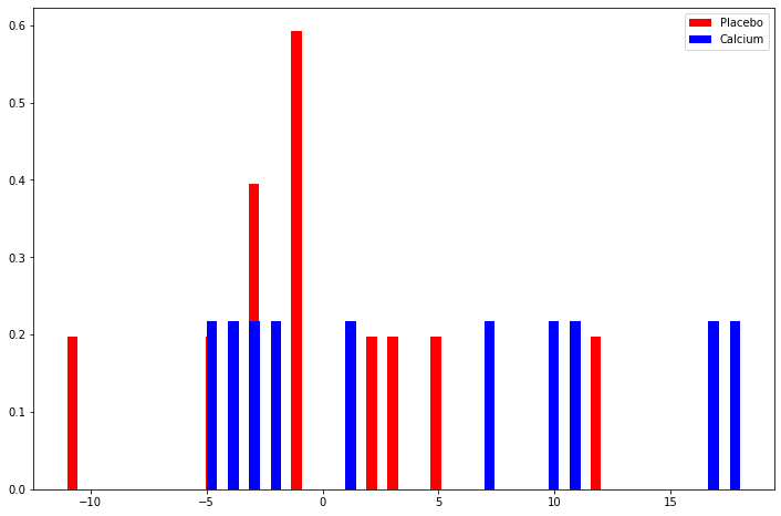
png
First, let’s calculate D – creating the empirical CDFs \(\hat{F}_1\) and \(\hat{F}_2\), and then testing the value of \(D\) for each possible \(x\) in the empirical distributions:
f1 = data[data['Treatment'] == 'Placebo']['Decrease'].to_numpy()
f2 = data[data['Treatment'] == 'Calcium']['Decrease'].to_numpy()

def f1_hat(x):
    return sum(f1 <= x) / len(f1)

def f2_hat(x):
    return sum(f2 <= x) / len(f2)

xx = np.linspace(min(data['Decrease']) - 1, max(data['Decrease']) + 1, 100)

fig, (ax1, ax2) = plt.subplots(2, sharex=True, figsize=(12, 8))
ax1.plot(xx, [f1_hat(x) for x in xx], color='red', label='Placebo empirical distribution')
ax1.plot(xx, [f2_hat(x) for x in xx], color='blue', label='Calcium empirical distribution')
ax1.legend(loc='upper left')

ax2.plot(xx, [abs(f1_hat(x) - f2_hat(x)) for x in xx], color='purple', label='|Placebo - Calcium|')
ax2.legend(loc='upper left')

plt.show()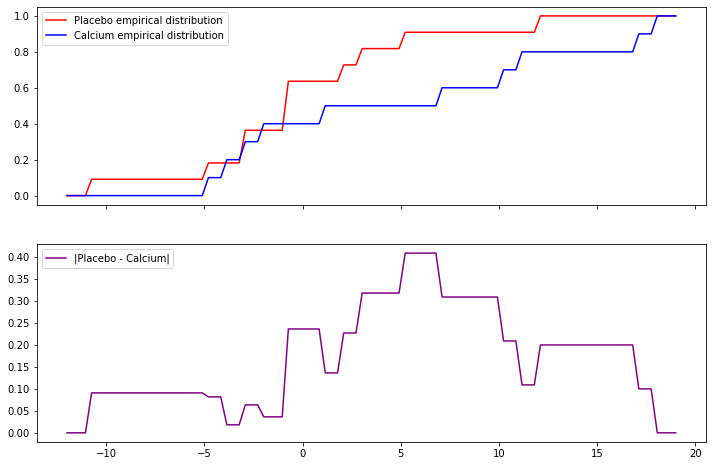
png
D = max([abs(f1_hat(x) - f2_hat(x)) for x in data['Decrease']])

n1 = len(f1)
n2 = len(f2)
test_statistic = np.sqrt(n1 * n2 / (n1 + n2)) * D

print('D: %.3f' % D)
print('Test statistic: %.3f' % test_statistic)
D: 0.409
Test statistic: 0.936Given that
\[ \begin{align} H(t) &= 1 - 2 \sum_{j=1}^\infty (-1)^{j-1} e^{-2j^2t^2} \end{align} \]
let’s create an approximation for \(H^{-1}(1 - \alpha)\) – so that we may find the p-value for \(\alpha\) such that $ D > H^{-1}(1 - ) $.
def H(t, xtol=1e-8):
    assert t != 0, "t must be non-zero"
    t2 = t * t
    j_max = int(np.ceil(np.sqrt(- np.log(xtol / 2) / (2 * t2) )))
    jj = np.arange(1, j_max+1)

    return 1 + 2 * sum((-1)**(jj) * np.exp(-2 * (jj**2) * t2))
# Let's plot some values for H(t)
tt = np.logspace(-3, 0.25, 100)
ht = [H(t) for t in tt]
plt.figure(figsize=(6, 4))
plt.plot(tt, ht)
plt.title('H(t)')
plt.show()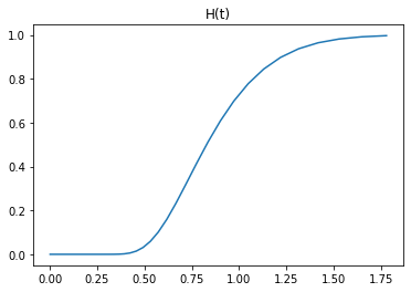
png
from scipy.optimize import minimize

def H_inv(q):
    def loss_function(x):
        return (H(x) - q)**2

    x0 = 1.0
    return minimize(loss_function, x0, method='nelder-mead').x
# Let's plot some values for H_inv(q)
qq = np.linspace(1e-5, 1 - 1e-5, 200)
xx = [H_inv(q) for q in qq]
plt.figure(figsize=(6, 4))
plt.plot(qq, xx)
plt.title(r'$H^{-1}(q)$')
plt.show()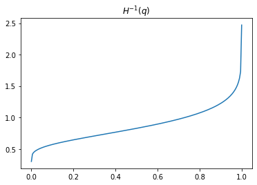
png
h_inv_test_statistic = H_inv(test_statistic)

print('Test statistic: \t\t%.3f' % test_statistic)
print('H^{-1}(test_statistic): \t%.3f' % h_inv_test_statistic)
Test statistic: 0.936
H^{-1}(test_statistic): 1.313Given that the inverse of the test statistic is greater than 1, we have that the test from Theorem 16.16 rejects the null hypothesis for any \(\alpha > 0\) – so it claims the distributions are distinct at any approximate \(\alpha\) level – so, by Theorem 16.15, they are associated.