AOS chapter15 Multivariate Models

15.1 Random Vectors

Multivariate models involve a random vector \(X\) of the form

\[X = \begin{pmatrix} X_1 \\ \vdots \\ X_k \end{pmatrix}\]

The mean of a random vector \(X\) is defined by

\[\mu = \begin{pmatrix} \mu_1 \\ \vdots \\ mu_k \end{pmatrix} = \begin{pmatrix} \mathbb{E}(X_1) \\ \vdots \\ \mathbb{E}(X_k) \end{pmatrix} \]

The covariance matrix \(\Sigma\) is defined to be

\[\Sigma = \mathbb{V}(X) = \begin{pmatrix} \mathbb{V}(X_1) & \text{Cov}(X_1, X_2) & \cdots & \text{Cov}(X_1, X_k) \\ \text{Cov}(X_2, X_1) & \mathbb{V}(X_2) & \cdots & \text{Cov}(X_2, X_k) \\ \vdots & \vdots & \ddots & \vdots \\ \text{Cov}(X_k, X_1) & \text{Cov}(X_k, X_2) & \cdots & \mathbb{V}(X_k) \end{pmatrix}\]

This is also called the variance matrix or the variance-covariance matrix.

Theorem 15.1. Let \(a\) be a vector of length \(k\) and let \(X\) be a random vector of the same length with mean \(\mu\) and variance \(\Sigma\). Then \(\mathbb{E}(a^T X) = a^T\mu\) and \(\mathbb{V}(a^T X) = a^T \Sigma a\). If \(A\) is a matrix with \(k\) columns then \(\mathbb{E}(AX) = A\mu\) and \(\mathbb{V}(AX) = A \Sigma A^T\).

Now suppose we have a random sample of \(n\) vectors:

\[ \begin{pmatrix}X_{11} \\ X_{21} \\ \vdots \\ X_{k1} \end{pmatrix}, \; \begin{pmatrix}X_{21} \\ X_{22} \\ \vdots \\ X_{k2} \end{pmatrix}, \; \cdots , \; \begin{pmatrix}X_{1n} \\ X_{2n} \\ \vdots \\ X_{kn} \end{pmatrix} \]

The sample mean \(\overline{X}\) is a vector defined by

\[\overline{X} = \begin{pmatrix} \overline{X}_1 \\ \vdots \\ \overline{X}_k \end{pmatrix}\]

where \(\overline{X}_i = n^{-1} \sum_{j = 1}^n X_{ij}\). The sample variance matrix is

\[ S = \begin{pmatrix} s_{11} & s_{12} & \cdots & s_{1k} \\ s_{12} & s_{22} & \cdots & s_{2k} \\ \vdots & \vdots & \ddots & \vdots \\ s_{1k} & s_{2k} & \cdots & s_{kk} \end{pmatrix} \]

where

\[s_{ab} = \frac{1}{n - 1} \sum_{j = 1}^n (X_{aj} - \overline{X}_a) (X_{bj} - \overline{X}_b)\]

It follows that \(\mathbb{E}(\overline{X}) = \mu\) and \(\mathbb{E}(S) = \Sigma\).

15.2 Estimating the Correlation

Consider \(n\) data points from a bivariate distribution

\[ \begin{pmatrix} X_{11} \\ X_{21}\end{pmatrix}, \; \begin{pmatrix} X_{12} \\ X_{22}\end{pmatrix}, \; \cdots \; \begin{pmatrix} X_{1n} \\ X_{1n}\end{pmatrix} \]

Recall that the correlation between \(X_1\) and \(X_2\) is

\[\rho = \frac{\mathbb{E}((X_1 - \mu) (X_2 - \mu_2))}{\sigma_1 \sigma_2}\]

The sample correlation (the plug-in estimator) is

\[\hat{\rho} = \frac{\sum_{i=1}^n (X_{1i} - \overline{X}_1)(X_{2i} - \overline{X}_2)}{s_1 s_2}\]

We can construct a confidence interval for \(\rho\) by applying the delta method as usual. However, it turns out that we get a more accurate confidence interval by first constructing a confidence interval for a function \(\theta = f(\rho)\) and then applying the inverse function \(f^{-1}\). The method, due to Fisher, is as follows. Define

\[f(r) = \frac{1}{2} \left( \log(1 + r) - \log(1 - r)\right) \]

and let \(\theta = f(\rho)\). The inverse of \(f\) is

\[g(z) \equiv f^{-1}(z) = \frac{e^{2z} - 1}{e^{2z} + 1}\]

Now do the following steps:

Approximate Confidence Interval for the Correlation

1. Compute

\[\hat{\theta} = f(\hat{\rho}) = \frac{1}{2} \left( \log(1 + \hat{\rho}) - \log(1 - \hat{\rho})\right) \]

2. Compute the approximate standard error of \(\hat{\theta}\) which can be shown to be

\[\hat{\text{se}}(\hat{\theta}) = \frac{1}{\sqrt{n - 3}} \]

3. An approximate \(1 - \alpha\) confidence interval for \(\theta = f(\rho)\) is

\[(a, b) \equiv \left(\hat{\theta} - \frac{z_{\alpha/2}}{\sqrt{n - 3}}, \; \hat{\theta} + \frac{z_{\alpha/2}}{\sqrt{n - 3}} \right)\]

4. Apply the inverse transformation \(f^{-1}(z)\) to get a confidence interval for \(\rho\):

\[ \left( \frac{e^{2a} - 1}{e^{2a} + 1}, \frac{e^{2b} - 1}{e^{2b} + 1} \right) \]

15.3 Multinomial

Review of Multinomial distribution: consider drawing a ball from an urn that has \(n\) balls of \(k\) colors. Let \(p = (p_1, \dots, p_k)\) where \(p_j \geq 0\) are the probabilities of drawing (with replacement) a ball of each color; \(\sum_j p_j = 1\). Draw \(n\) times and let \(X = (X_1, \dots, X_n)\) where \(X_j\) is the number of times that color \(j\) appeared; so \(\sum_k X_k = n\). We say \(X\) has a Multinomial(\(n\), \(p\)) distribution. The probability function is

\[ f(x; p) = \binom{n}{x_1 \dots x_k} p_1^{x_1}\dots p_k^{x_k}\]

where

\[ \binom{n}{x_1 \dots x_k} = \frac{n!}{x_1! \dots x_k!} \]

Theorem 15.2. Let \(X \sim \text{Multinomial}(n, p)\). Then the marginal distribution of \(X_j\) is \(X_j \sim \text{Binomial}(n, p_j)\). The mean and variance of \(X\) are

\[\mathbb{E}(X) = \begin{pmatrix} np_1 \\ \vdots \\ np_k \end{pmatrix}\]

and

\[\mathbb{V}(X) = \begin{pmatrix} np_1(1 - p_1) & -np_1p_2 & \cdots & -np_1p_k \\ -np_1p_2 & np_2(1 - p_2) & \cdots & -np_2p_k \\ \vdots & \vdots & \ddots & \vdots \\ -np_1p_k & -np_2p_k & \cdots & -np_k(1 - p_k) \end{pmatrix}\]

Proof. That \(X_j \sim \text{Bimomial}(n, p_j)\) follows easily. Hence \(\mathbb{E}(X_j) = np_j\) and \(\mathbb{V}(X_j) = np_j(1 - p_j)\).

To compute \(\text{Cov}(X_i, X_j)\), notice that \(X_i + X_j \sim \text{Binomial}(n, p_i + p_j)\), so \(\mathbb{V}(X_i + X_j) = n (p_i + p_j) (1 - p_i - p_j)\). On the other hand, decomposing the sum of the random variables on the variance,

\[ \begin{align} \mathbb{V}(X_i + X_j) &= \mathbb{V}(X_i) + \mathbb{V}(X_j) + 2 \text{Cov}(X_i, X_j) \\ &= np_i(1 - p_i) + np_j(1 - p_j) + 2 \text{Cov}(X_i, X_j) \end{align} \]

Equating both expressions and isolating the covariance we get \(\text{Cov}(X_i, X_j) = -np_ip_j\).

Theorem 15.3. The maximum likelihood estimator of \(p\) is

\[\hat{p} = \begin{pmatrix} \hat{p}_1 \\ \vdots \\ \hat{p}_k \end{pmatrix} = \begin{pmatrix} \frac{X_1}{n} \\ \vdots \\ \frac{X_k}{n} \end{pmatrix} = \frac{X}{n} \]

Proof. The log-likelihood (ignoring a constant) is \(\ell(p) = \sum_j X_j \log p_j\). When we maximize it we need to be careful to enforce the constraint that \(\sum_j p_j = 1\). Using Lagrange multipliers, instead we maximize

\[A(p) = \sum_{j=1}^k X_j \log p_j + \lambda \left( \sum_{j=1}^k p_j - 1 \right)\]

But

\[\frac{\partial A(p)}{\partial p_j} = \frac{X_j}{p_j} + \lambda\]

Setting it to zero we get \(\hat{p}_j = - X_j / \lambda\). Since \(\sum_j \hat{p}_j = 1\) we get \(\lambda = -n\) and so \(\hat{p}_j = X_j / n\), which is our result.

Next we want the variance of the MLE. The direct approach is to compute the variance matrix of \(\hat{p}\) directly: \(\mathbb{V}(\hat{p}) = \mathbb{V}(X / n) = n^{-2} \mathbb{V}(X)\), so

\[\mathbb{V}(\hat{p}) = \frac{1}{n} \begin{pmatrix} p_1(1 - p_1) & -p_1p_2 & \cdots & -p_1p_k \\ -p_1p_2 & p_2(1 - p_2) & \cdots & -p_2p_k \\ \vdots & \vdots & \ddots & \vdots \\ -p_1p_k & -p_2p_k & \cdots & p_k(1 - p_k) \end{pmatrix}\]

15.4 Multivariate Normal

Let’s recall the definition of the multivariate normal. Let

\[ Z = \begin{pmatrix} Z_1 \\ \vdots \\ Z_k \end{pmatrix} \]

where \(Z_1, \dots, Z_k \sim N(0, 1)\) are independent. The density of \(Z\) is

\[ f(z) = \frac{1}{(2\pi)^{k / 2}} \exp \left\{ -\frac{1}{2} \sum_{j=1}^k z_j^2 \right\} = \frac{1}{(2\pi)^{k / 2}} \exp \left\{ -\frac{1}{2} z^T z \right\}\]

The variance matrix of \(Z\) is the identity matrix \(I\). We write \(Z \sim N(0, I)\) where it is understood that \(0\) is a vector of \(k\) zeroes. We say \(Z\) has a standard multivariate Normal distribution.

More generally, a vector \(X\) has a multivariate Normal distribution, denoted by \(X \sim N(\mu, \Sigma)\), if its density is

\[ f(x; \mu, \Sigma) = \frac{1}{(2 \pi)^{k / 2} \text{det}(\Sigma)^{1/2}} \exp \left\{ -\frac{1}{2} (x - \mu)^T \Sigma^{-1} (x - \mu)\right\}\]

where \(\mu\) is a vector of length \(k\) and \(\Sigma\) is a \(k \times k\) symmetric, positive definite matrix. Then \(\mathbb{E}(X) = \mu\) and \(\mathbb{V}(X) = \Sigma\). Setting \(\mu = 0\) and \(\Sigma = I\) gives back the standard Normal.

Theorem 15.4. The following properties hold:

1. If \(Z \sim N(0, 1)\) and \(X = \mu + \Sigma^{1/2} Z\) then \(X \sim N(\mu, \Sigma)\).

2. If \(X \sim N(\mu, \Sigma)\), then \(\Sigma^{-1/2}(X - \mu) \sim N(0, 1)\).

3. If \(X \sim N(\mu, \Sigma)\) and \(a\) is a vector with the same length as \(X\), then \(a^T X \sim N(a^T \mu, a^T \Sigma a)\).

4. Let \(V = (X - \mu)^T \Sigma^{-1} (X - \mu)\). Then \(V \sim \xi_k^2\).

Suppose we partition a random Normal vector \(X\) into two parts \(X = (X_a, X_b)\). We can similarly partition the mean \(\mu = (\mu_a, \mu_b)\) and the variance

\[\Sigma = \begin{pmatrix} \Sigma_{aa} & \Sigma_{ab} \\ \Sigma_{ba} & \Sigma_{bb} \end{pmatrix}\]

Theorem 15.5. Let \(X \sim N(\mu, \Sigma)\). Then:

1. The marginal distribution of \(X_a\) is \(X_a \sim N(\mu_a, \Sigma_{aa})\).
2. The conditional distribution of \(X_b\) given \(X_a = x_a\) is

\[ X_b | X_a = x_a \sim N(\mu(x_a), \Sigma(x_a))\]

where

\[ \begin{align} \mu(x_a) &= \mu_b + \Sigma_{ba} \Sigma_{aa}^{-1} (x_a - \mu_a) \\ \Sigma(x_a) &= \Sigma_{bb} - \Sigma_{ba}\Sigma_{aa}^{-1}\Sigma_{ab} \end{align} \]

Theorem 15.6. Given a random sample of size \(n\) from a \(N(\mu, \Sigma)\), the log-likelihood (up to a constant not depending on \(\mu\) or \(\Sigma\)) is given by

\[\ell(\mu, \Sigma) = -\frac{n}{2} (\overline{X} - \mu)^T \Sigma^{-1} (\overline{X} - \mu) - \frac{n}{2} \text{tr} \left( \Sigma^{-1}S \right) - \frac{n}{2} \log \text{det} \left( \Sigma \right) \]

The MLE is

\[ \hat{\mu} = \overline{X} \quad \text{and} \quad \hat{\Sigma} = \left( \frac{n - 1}{n} \right) S\]

15.5 Appendix

Proof of Theorem 15.6. Let the \(i\)-th random vector be \(X^i\). The log-likelihood is

\[\ell(\mu, \Sigma) = \sum_{i = 1}^n f(X^i; \mu, \Sigma) = -\frac{kn}{2} \log ( 2\pi ) - \frac{n}{2} \log \text{det} \left( \Sigma \right) - \frac{1}{2} \sum_{i=1}^n (X^i - \mu)^T \Sigma^{-1} (X^i - \mu) \]

Now,

\[ \begin{align} \sum_{i=1}^n (X^i - \mu)^T \Sigma^{-1} (X^i - \mu) &= \sum_{i=1}^n \left[ (X^i - \overline {X}) + (\overline{X} - \mu) \right]^T \Sigma^{-1} \left[(X^i - \overline{X}) + (\overline{X} - \mu) \right] \\ &= \sum_{i=1}^n \left[(X^i - \overline{X})^T\Sigma^{-1}(X^i - \overline{X})\right] + n (\overline{X} - \mu)^T \Sigma^{-1} (\overline{X} - \mu) \end{align} \]

since \(\sum_i (X^i - \overline{X})^T \Sigma^{-1} (\overline{X} - \mu) = 0\). Also, \((X^i - \mu)^T \Sigma^T (X^i - \mu)\) is a scalar, so

\[ \begin{align} \sum_{i=1}^n (X^i - \mu)^T \Sigma^{-1} (X^i - \mu) &= \sum_{i=1}^n \text{tr} \left[ (X^i - \mu)^T \Sigma^{-1} (X^i - \mu)\right] \\ &= \sum_{i=1}^n \text{tr} \left[ \Sigma^{-1} (X^i - \mu) (X^i - \mu)^T \right] \\ &= \text{tr} \left[ \Sigma^{-1} \sum_{i=1}^n (X^i - \mu) (X^i - \mu) ^T \right] \\ &= n \; \text{tr} \left[ \Sigma^{-1} S\right] \end{align} \]

so the conclusion follows.

15.6 Exercises

Exercise 15.6.1. Prove Theorem 15.1.

Let \(a\) be a vector of length \(k\) and let \(X\) be a random vector of the same length with mean \(\mu\) and variance \(\Sigma\). Then \(\mathbb{E}(a^T X) = a^T\mu\) and \(\mathbb{V}(a^T X) = a^T \Sigma a\). If \(A\) is a matrix with \(k\) columns then \(\mathbb{E}(AX) = A\mu\) and \(\mathbb{V}(AX) = A \Sigma A^T\).

Solution.

For the vector version of the theorem, we have:

\[\mathbb{E}(a^T X) = \mathbb{E}\left( \sum_{i=1}^k a_i X_i \right) = \sum_{i=1}^k a_i \mathbb{E}(X_i) = \sum_{i=1}^k a_i \mu_i = a^T \mu \]

\[\mathbb{V}(a^T X) = \mathbb{V}\left( \sum_{i=1}^k a_i X_i \right) = \sum_{i=1}^k \sum_{j=1}^k a_i a_j \text{Cov} (X_i, X_j) = \sum_{i=1}^k a_i \left( \sum_{j=1}^k \text{Cov}(X_i, X_j) a_j \right) = \sum_{i=1}^k a_i \Big( \Sigma a \Big)_i = a^T \Sigma a\]

For the matrix version of the theorem, consider the \(r\) rows of \(A\) as vectors, separately, \(a^1, \dots, a^k\):

\[ A = \begin{pmatrix} \cdots & a^1 & \cdots \\ \cdots & a^2 & \cdots \\ \vdots & \vdots & \vdots \\ \cdots & a^r & \cdots \end{pmatrix}\]

Then,

\[ \mathbb{E}(AX) = \begin{pmatrix} \mathbb{E}(a^1 X) \\ \mathbb{E}(a^2 X) \\ \vdots \\ \mathbb{E}(a^r X) \end{pmatrix} = \begin{pmatrix} a^1 \mu \\ a^2 \mu \\ \vdots \\ a^r \mu \end{pmatrix} = A\mu \]

Finally, looking at the \(i\)-th term of \(AX\),

\[(AX)_i = \sum_{s=1}^k a_{is} X_s = a^i X\]

so, by the vector version of the theorem, \(\mathbb{V}((AX)_i) = (a^i)^T \Sigma a^i\). Applying this to every element:

\[\mathbb{V}(AX) = \begin{pmatrix} \mathbb{V}((AX)_1) \\ \mathbb{V}((AX)_2) \\ \vdots \\ \mathbb{V}((AX)_r) \end{pmatrix} = \begin{pmatrix} \mathbb{V}(a^1 X) \\ \mathbb{V}(a^2 X) \\ \vdots \\ \mathbb{V}(a^r X) \end{pmatrix} = \begin{pmatrix} (a^1)^T \Sigma a^1 \\ (a^2)^T \Sigma a^2 \\ \vdots \\ (a^r)^T \Sigma a^r \end{pmatrix} = A \Sigma A^T\]

Exercise 15.6.2. Find the Fisher information matrix for the MLE of a Multinomial.

Solution.

The probability mass function for a Multinomial distribution is:

\[ f(X; p) = \binom{n}{X_1 \dots X_k} p_1^{X_1} \dots p_k^{X_k} = \frac{n!}{X_1! \dots X_k!} p_1^{X_1} \dots p_k^{X_k}\]

so the log-likelihood (ignoring a constant) is

\[ \ell_n(p) = \sum_{i=1}^k X_i \log p_i\]

The partial derivatives are:

\[ \begin{align} H_{ii} = \frac{\partial^2 \ell_n(p)}{\partial^2 p_i} &= -\frac{X_i}{p_i^2} \\ H_{ij} = \frac{\partial^2 \ell_n(p)}{\partial p_i \partial p_j} &= 0 \; \text{for } i \neq j \end{align} \]

so \(\mathbb{E}(H_{ii}) = - n/p_i\), and the Fisher Information Matrix is:

\[I_n(p) = n \begin{pmatrix} \frac{1}{p_1} & 0 & \cdots & 0 \\ 0 & \frac{1}{p_2} & \cdots & 0 \\ \vdots & \vdots & \ddots & \vdots \\ 0 & 0 & \cdots & \frac{1}{p_k} \end{pmatrix}\]

Note, however, that the variance is not the inverse matrix of \(I_n(p)\), and further, that, \(\mathbb{V}(X)\) is not invertible.

Exercise 15.6.3. Prove Theorem 15.5.

Let \(X \sim N(\mu, \Sigma)\). Then:

1. The marginal distribution of \(X_a\) is \(X_a \sim N(\mu_a, \Sigma_{aa})\).
2. The conditional distribution of \(X_b\) given \(X_a = x_a\) is

\[ X_b | X_a = x_a \sim N(\mu(x_a), \Sigma(x_a))\]

where

\[ \begin{align} \mu(x_a) &= \mu_b + \Sigma_{ba} \Sigma_{aa}^{-1} (x_a - \mu_a) \\ \Sigma(x_a) &= \Sigma_{bb} - \Sigma_{ba}\Sigma_{aa}^{-1}\Sigma_{ab} \end{align} \]

Solution.

The marginal distribution result is immediate: for any given sample drawn from the distribution, collect only the first \(k\) dimensions of the sample vector, where \(k\) is the number of dimensions of \(X_a\). The resulting distribution will be multivariate normal, with mean and variance given by getting the first \(k\) dimensions of \(\mu\) and \(\Sigma\).

For the conditional distribution result, let \(A = -\Sigma_{ba} \Sigma_{aa}^{-1}\) and \(z = x_b + A x_a\). We have:

\[\begin{align} \text{Cov}(z, x_a) &= \text{Cov}(x_b, x_a) + \text{Cov}(A x_a, x_a) \\ &= \Sigma_{ba} + A \mathbb{V}(x_a) \\ &= \Sigma_{ba} - \Sigma_{ba} \Sigma_{aa}^{-1} \Sigma_{aa} \\ &= 0 \end{align}\]

so \(z\) and \(x_a\) are uncorrelated (and since they are jointly normal, they are also independent). We then have:

\[\begin{align} \mathbb{E}(x_b | x_a) &= \mathbb{E}(z - A x_a | x_a) \\ &= \mathbb{E}(z | x_a) - \mathbb{E}(A x_a | x_a) \\ &= \mathbb{E}(z) - A x_a \\ &= \mu_b + A \mu_a - A x_a \\ &= \mu_b + \Sigma_{ba} \Sigma_{aa}^{-1} (x_a - \mu_a) \end{align}\]

For the covariance matrix,

\[\begin{align} \mathbb{V}(x_b | x_a) &= \mathbb{V}(z - A x_a | x_a) \\ &= \mathbb{V}(z | x_a) - \mathbb{V}(A x_a | x_a) - A \text{Cov}(z, -x_a) - \text{Cov}(z, -x_a) A^T \\ &= \mathbb{V}(z | x_a) - 0 - A \cdot 0 - 0 \cdot A \\ &= \mathbb{V}(z) \\ &= \mathbb{V}(x_b + A x_a) \\ &= \mathbb{V}(x_b) + A \mathbb{V}(x_a) A^T + A \text{Cov}(x_a, x_b) + \text{Cov}(x_b, x_a) A^T \\ &= \Sigma_{bb} + (- \Sigma_{ba} \Sigma_{aa}^{-1}) \Sigma_{aa} (- \Sigma_{ba} \Sigma_{aa}^{-1})^T + (- \Sigma_{ba} \Sigma_{aa}^{-1}) \Sigma_{ab} + \Sigma_{ba} (- \Sigma_{ba} \Sigma_{aa}^{-1})^T \\ &= \Sigma_{bb} + \Sigma_{ba} \Sigma_{aa}^{-1} \Sigma_{aa} \Sigma_{aa}^{-1} \Sigma_{ab} - 2 \Sigma_{ba}\Sigma_{aa}^{-1}\Sigma_{ab} \\ &= \Sigma_{bb} - \Sigma_{ba}\Sigma_{aa}^{-1}\Sigma_{ab} \end{align}\]

Reference: Macro (https://stats.stackexchange.com/users/4856/macro), Deriving the conditional distributions of a multivariate normal distribution, URL (version: 2015-06-18): https://stats.stackexchange.com/q/30600

Exercise 15.6.4 (Computer Experiment). Write a function to generate \(\text{nsim}\) observations from a \(\text{Multinomial}(n, p)\) distribution.

Solution. Let’s use the combinatoric interpretation of the distribution: Drawing \(n\) times, with replacement, from an urn with different ball colors, where the probability of obtaining balls of color \(i\) is \(p_i\).

import numpy as np

def multinomial_observations(n, p, nsim=1):
    cumulative_probabilities = np.cumsum(p)
    
    # Ensure probabilities add up to 1 (approximately)
    assert abs(cumulative_probabilities[-1] - 1) < 1e-8, "Probabilities should add up to 1"
    
    def get_observation():
        counts = np.zeros(cumulative_probabilities.size).astype(int)
        rvs = np.random.uniform(size=n)
        for i in range(n):
            counts[np.argmin(rvs[i] > cumulative_probabilities)] += 1

        return counts
    
    return np.array([get_observation() for _ in range(nsim)])

# Sample usage
import matplotlib.pyplot as plt
%matplotlib inline

obs = multinomial_observations(n=500, p=[0.5, 0.3, 0.2], nsim=1000)

plt.figure(figsize=(12, 8))
plt.hist(obs[:, 0], density=True, bins=25, histtype='step', color='red', label='p = 0.5')
plt.hist(obs[:, 1], density=True, bins=25, histtype='step', color='green', label='p = 0.3')
plt.hist(obs[:, 2], density=True, bins=25, histtype='step', color='blue', label='p = 0.2')
plt.legend(loc='upper right')
plt.show()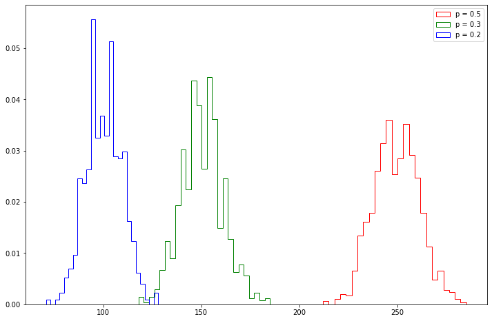

png

obs

array([[266, 131, 103],
       [258, 151,  91],
       [252, 146, 102],
       ...,
       [268, 161,  71],
       [241, 165,  94],
       [256, 142, 102]])

Exercise 15.6.5 (Computer Experiment). Write a function to generate \(\text{nsim}\) observations from a Multivariate normal with given mean \(\mu\) and covariance matrix \(\Sigma\).

Solution. Let’s construct our samples based on samples of a standard multivariate normal \(Z \sim N(0, I)\), by making \(X = \mu + \Sigma^{1/2} Z\).

box_muller

A transformation which transforms from a two-dimensional continuous uniform distribution to a two-dimensional bivariate normal distribution (or complex normal distribution). If \(x_1\) and \(x_2\) are uniformly and independently distributed between \(0\) and \(1\), then \(z_1\) and \(z_2\) as defined below have a normal distribution with mean \(\mu=0\) and variance \(\sigma^2=1\).

\[z_1=\sqrt{-2\ln{x_1}}\cos(2\pi x_2)\] \[z_2=\sqrt{-2\ln{x_1}}\sin(2\pi x_2)\] This can be verified by solving for \(x_1\) and \(x_2\),

\[x_1=e^{-(z_1^2+z_2^2)/2}\] \[x_2=\frac{1}{2\pi}\tan^{-1}\left(\frac{z_2}{z_1}\right)\]

Taking the Jacobian yields

\[\frac{\partial(x_1,x_2)}{\partial(z_1,z_2)}=\begin{bmatrix} \frac{\partial x_1}{\partial z_1} & \frac{\partial x_1}{\partial z_2}\\ \frac{\partial x_2}{\partial z_1} & \frac{\partial x_2}{\partial z_2}\\ \end{bmatrix}\\ =-\left[\frac{1}{\sqrt{2\pi}}e^{-z_1^2/2}\right]\left[\frac{1}{\sqrt{2\pi}}e^{-z_2^2/2}\right] \]

import numpy as np

def multivariate_normal_observations(mu, sigma, nsim=1):
    mu_array = np.array(mu)
    sigma_array = np.array(sigma)
    
    assert len(mu_array.shape) == 1, "mu should be a vector"
    k = mu_array.shape[0]
    
    assert sigma_array.shape == (k, k), "sigma should be a square matrix with same length as mu"
    
    # Do the eigenvalue decomposition, then get U D^{1/2} as Sigma^{1/2}
    U, D, V = np.linalg.svd(sigma_array)
    sigma_sqrt = U @ np.diag(np.sqrt(D))
    
    # Let's write our own random normal generator for fun, rather than use np.random.normal
    # Strategy: Use Box-Muller to transform two random uniform variables in (0, 1) 
    # into two standard normals
    def random_normals(size):

        def box_muller(u1, u2):
            R = np.sqrt(-2 * np.log(u1))
            theta = 2 * np.pi * u2

            z0 = R * np.cos(theta)
            z1 = R * np.sin(theta)

            return z0, z1

        def normal_generator(uniform_generator):
            while True:
                z0, z1 = box_muller(next(uniform_generator), next(uniform_generator))
                yield z0
                yield z1

        def random_generator(batch_size):
            while True:
                for v in np.random.uniform(size=batch_size):
                    yield v

        result = np.empty(size)
        gen = normal_generator(random_generator(batch_size=min(size, 1024)))
        for i in range(size):
            result[i] = next(gen)

        return result

    def get_observation():
        z = random_normals(k)
        return mu_array + sigma_sqrt @ z
    
    return np.array([get_observation() for _ in range(nsim)])

# Sample usage
import matplotlib.pyplot as plt
%matplotlib inline

mu = [1, 3]
sigma = [[2, 1], [1, 2]]
obs = multivariate_normal_observations(mu, sigma, nsim=5000)

plt.figure(figsize=(12, 8))
plt.hexbin(obs[:, 0], obs[:, 1], cmap=plt.cm.Reds)
plt.show()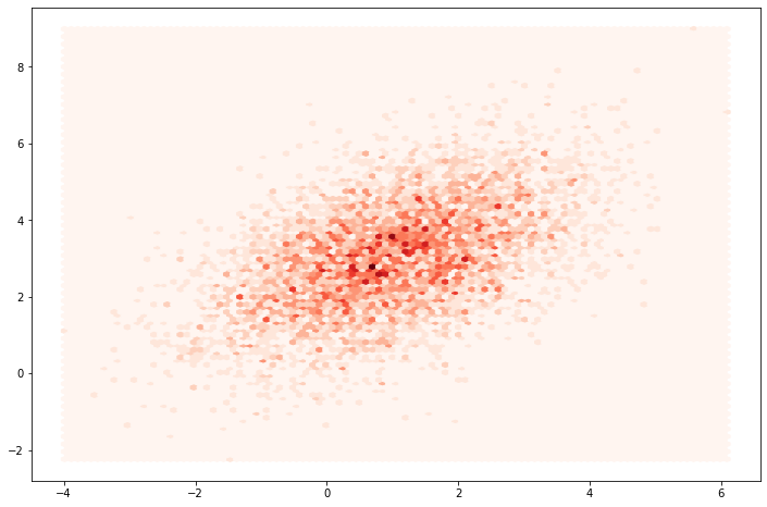

png

Exercise 15.6.6 (Computer Experiment). Generate 1000 random vectors from a \(N(\mu, \Sigma)\) distribution where

\[ \mu = \begin{pmatrix} 3 \\ 8\end{pmatrix} , \quad \Sigma = \begin{pmatrix} 2 & 6 \\ 6 & 2 \end{pmatrix}\]

Plot the simulation as a scatterplot. Find the distribution of \(X_2 | X_1 = x_1\) using theorem 15.5. In particular, what is the formula for \(\mathbb{E}(X_2 | X_1 = x_1)\)? Plot \(\mathbb{E}(X_2 | X_1 = x_1)\) on your scatterplot. Find the correlation \(\rho\) between \(X_1\) and \(X_2\). Compare this with the sample correlations from your simulation. Find a 95% confidence interval for \(\rho\). Estimate the covariance matrix \(\Sigma\).

Solution.

The provided \(\Sigma\) matrix has negative eigenvalues. We will instead use the following matrix:

\[ \Sigma = \begin{pmatrix} 6 & 2 \\ 2 & 6\end{pmatrix}\]

# Generate 1000 vectors
mu = [3, 8]
sigma = [[6, 2], [2, 6]]
obs = multivariate_normal_observations(mu, sigma, nsim=1000)

# Using numpy to generate observations:
#obs = np.random.multivariate_normal(mu, sigma, size=1000)

# Using scipy to generate observations:
#obs = scipy.stats.multivariate_normal.rvs(mean=mu, cov=sigma, size=1000)

x, y = obs[:, 0], obs[:, 1]

# Plot scatterplot
plt.figure(figsize=(12, 8))
plt.scatter(x, y)
plt.show()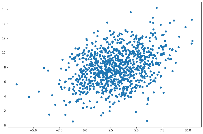

png

From theorem 15.5,

\[ X_2 | X_1 = x_1 \sim N(\mu(x_1), \Sigma(x_1))\]

where

\[ \begin{align} \mu(x_1) &= \mu_2 + \Sigma_{21} \Sigma_{11}^{-1} (x_1 - \mu_1) \\ \Sigma(x_1) &= \Sigma_{22} - \Sigma_{21}\Sigma_{11}^{-1}\Sigma_{12} \end{align} \]

Replacing the given values,

\[ \begin{align} \mu(x_1) &= 8 + 2 \cdot 6^{-1} (x_1 - 3) = \frac{1}{3} x_1 + \frac{22}{3}\\ \Sigma(x_1) &= 6 - 2 \cdot 6^{-1} \cdot 2 = \frac{16}{3} \end{align} \]

# Plot scatterplot + line
f = lambda x: x/3 + 22/3

plt.figure(figsize=(12, 8))
plt.scatter(x, y)
plt.plot([-6, 10], [f(-6), f(10)], color='red')
plt.show()

png

The correlation \(\rho\) between \(X_1\) and \(X_2\) is:

\[ \rho = \frac{\text{Cov}(X_1, X_2)}{\sigma_{X_1} \sigma_{X_2}} = \frac{1}{3}\]

The estimated correlation \(\rho\) between \(X_1\) and \(X_2\) is:

\[ \hat{\rho} = \frac{\sum_i (X_{1i} - \overline{X}_1)(X_{2i} - \overline{X}_2)}{s_{X_1} s_{X_2}}\]

rho_hat = np.corrcoef(x, y)[0, 1]
print("Estimated correlation: %.3f" % rho_hat)

Estimated correlation: 0.342

We will use the provided process to estimate a confidence interval for the correlation:

Approximate Confidence Interval for the Correlation

1. Compute

\[\hat{\theta} = f(\hat{\rho}) = \frac{1}{2} \left( \log(1 + \hat{\rho}) - \log(1 - \hat{\rho})\right) \]

2. Compute the approximate standard error of \(\hat{\theta}\) which can be shown to be

\[\hat{\text{se}}(\hat{\theta}) = \frac{1}{\sqrt{n - 3}} \]

3. An approximate \(1 - \alpha\) confidence interval for \(\theta = f(\rho)\) is

\[(a, b) \equiv \left(\hat{\theta} - \frac{z_{\alpha/2}}{\sqrt{n - 3}}, \; \hat{\theta} + \frac{z_{\alpha/2}}{\sqrt{n - 3}} \right)\]

4. Apply the inverse transformation \(f^{-1}(z)\) to get a confidence interval for \(\rho\):

\[ \left( \frac{e^{2a} - 1}{e^{2a} + 1}, \frac{e^{2b} - 1}{e^{2b} + 1} \right) \]

from scipy.stats import norm

theta_hat = (np.log(1 + rho_hat) - np.log(1 - rho_hat)) / 2
se_theta_hat = 1 / np.sqrt(1000 - 3)
z = norm.ppf(0.975)
a, b = theta_hat - z * se_theta_hat, theta_hat + z * se_theta_hat
f_inv = lambda x: (np.exp(2*x) - 1) / (np.exp(2*x) + 1)
confidence_interval = (f_inv(a), f_inv(b))

print('95%% confidence interval: %.3f, %.3f' % confidence_interval)

95% confidence interval: 0.286, 0.395

The sample covariance matrix is:

\[ \hat{\Sigma} = \frac{1}{n} S = \frac{1}{n} \sum_{i=1}^n (X_i - \overline{X})(X_i - \overline{X})^T \]

import numpy as np
mu_hat = np.array([x.mean(), y.mean()])
xx = np.concatenate((x.reshape(-1, 1), y.reshape(-1, 1)), axis=1)
sigma_hat = (xx - mu_hat).T @ (xx - mu_hat) / 1000

sigma_hat

array([[5.67452097, 1.90244085],
       [1.90244085, 5.82662727]])

Exercise 15.6.7 (Computer Experiment). Generate 100 random vectors from a multivariate Normal with mean \((0, 2)^T\) and variance

\[ \begin{pmatrix} 1 & 3 \\ 3 & 1 \end{pmatrix} \]

Find a 95% confidence interval for the correlation \(\rho\). What is the true value of \(\rho\)?

Solution.

The provided matrix, yet again, has negative eigenvalues. Let’s instead use:

\[\Sigma = \begin{pmatrix} 3 & 1 \\ 1 & 3 \end{pmatrix}\]

# Generate 100 vectors
n = 100
mu = [0, 2]
sigma = [[3, 1], [1, 3]]
obs = multivariate_normal_observations(mu, sigma, nsim=n)
x, y = obs[:, 0], obs[:, 1]

# Plot scatterplot
plt.figure(figsize=(12, 8))
plt.scatter(x, y)
plt.show()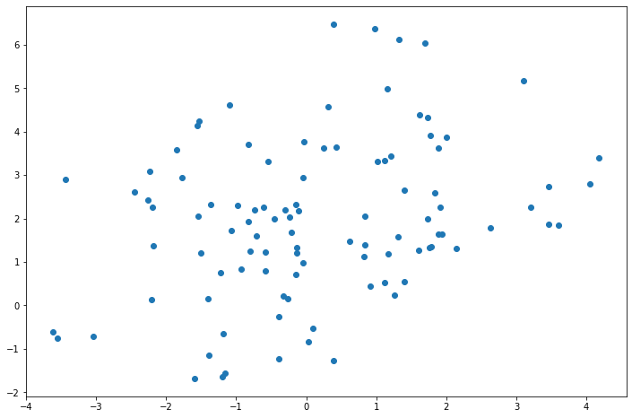

png

# Find 95% confidence interval
from scipy.stats import norm

rho_hat = np.corrcoef(x, y)[0, 1]
theta_hat = (np.log(1 + rho_hat) - np.log(1 - rho_hat)) / 2
se_theta_hat = 1 / np.sqrt(n - 3)
z = norm.ppf(0.975)
a, b = theta_hat - z * se_theta_hat, theta_hat + z * se_theta_hat
f_inv = lambda x: (np.exp(2*x) - 1) / (np.exp(2*x) + 1)
confidence_interval = (f_inv(a), f_inv(b))

print('95%% confidence interval: %.3f, %.3f' % confidence_interval)

95% confidence interval: 0.116, 0.474

True value of \(\rho\):

\[ \rho = \frac{\text{Cov}(X_1, X_2)}{\sigma_{X_1} \sigma_{X_2}} = \frac{1}{3}\]