14. Linear Regression
Regression is a method for studying the relationship between a response variable \(Y\) and a covariates \(X\). The covariate is also called a predictor variable or feature. Later we will generalize and allow for more than one covariate. The data are of the form
\[ (Y_1, X_1), \dots, (Y_n, X_n) \]
One way to summarize the relationship between \(X\) and \(Y\) is through the regression function
\[ r(x) = \mathbb{E}(Y | X = x) = \int y f(y | x) dy \]
Most of this chapter is concerned with estimating the regression function.
14.1 Simple Linear Regression
The simplest version of regression is when \(X_i\) is simple (a scalar, not a vector) and \(r(x)\) is assumed to be linear:
\[r(x) = \beta_0 + \beta_1 x\]
This model is called the simple linear regression model. Let \(\epsilon_i = Y_i - (\beta_0 + \beta_1 X_i)\). Then:
\[ \begin{align} \mathbb{E}(\epsilon_i | Y_i) &= \mathbb{E}(Y_i - (\beta_0 + \beta_1 X_i) | X_i)\\ &= \mathbb{E}(Y_i | X_i) - (\beta_0 + \beta_1 X_i)\\ &= r(X_i) - (\beta_0 + \beta_1 X_i)\\ &= 0 \end{align} \]
Let \(\sigma^2(x) = \mathbb{V}(\epsilon_i | X_i = x)\). We will make the further simplifying assumption that \(\sigma^2(x) = \sigma^2\) does not depend on \(x\).
The Linear Regression Model
\[Y_i = \beta_0 + \beta_1 X_i + \epsilon_i\]
where \(\mathbb{E}(\epsilon_i | X_i) = 0\) and \(\mathbb{V}(\epsilon_i | X_i) = \sigma^2\).
The unknown models in the parameter are the intercept \(\beta_0\), the slope \(\beta_1\) and the variance \(\sigma^2\). Let \(\hat{\beta_0}\) and \(\hat{\beta_1}\) denote the estimates of \(\beta_0\) and \(\beta_1\). The fitted line is defined to be
\[\hat{r}(x) = \hat{\beta}_0 + \hat{\beta}_1 x\]
The predicted values or fitted values are \(\hat{Y}_i = \hat{r}(X_i)\) and the residuals are defined to be
\[\hat{\epsilon}_i = Y_i - \hat{Y}_i = Y_i - (\hat{\beta}_0 + \hat{\beta}_1 X_i)\]
The residual sum of squares or RSS is defined by
\[ \text{RSS} = \sum_{i=1}^n \hat{\epsilon}_i^2\]
The quantity RSS measures how well the fitted line fits the data.
The least squares estimates are the values \(\hat{\beta}_0\) and \(\hat{\beta}_1\) that minimize \(\text{RSS} = \sum_{i=1}^n \hat{\epsilon}_i^2\).
Theorem 14.4. The least square estimates are given by
\[ \begin{align} \hat{\beta}_1 &= \frac{\sum_{i=1}^n (X_i - \overline{X}_n) (Y_i - \overline{Y}_n)}{\sum_{i=1}^n (X_i - \overline{X}_n)^2}\\ \hat{\beta}_0 &= \overline{Y}_n - \hat{\beta}_1 \overline{X}_n \end{align} \]
An unbiased estimate of \(\sigma^2\) is
\[ \hat{\sigma}^2 = \left( \frac{1}{n - 2} \right) \sum_{i=1}^n \hat{\epsilon}_i^2 \]
14.2 Least Squares and Maximum Likelihood
Suppose we add the assumption that \(\epsilon_i | X_i \sim N(0, \sigma^2)\), that is,
\(Y_i | X_i \sim N(\mu_i, \sigma_i^2)\)
where \(\mu_i = \beta_0 + \beta_i X_i\). The likelihood function is
\[ \begin{align} \prod_{i=1}n f(X_i, Y_i) &= \prod_{i=1}^n f_X(X_i) f_{Y|X}(Y_i | X_i)\\ &= \prod_{i=1}^n f_X(X_i) \times \prod_{i=1}^n f_{Y|X}(Y_i | X_i) \\ &= \mathcal{L}_1 \times \mathcal{L}_2 \end{align} \]
where \(\mathcal{L}_1 = \prod_{i=1}^n f_X(X_i)\) and \(\mathcal{L}_2 = \prod_{i=1}^n f_{Y|X}(Y_i | X_i)\).
The term \(\mathcal{L}_1\) does not involve the parameters \(\beta_0\) and \(\beta_1\). We shall focus on the second term \(\mathcal{L}_2\) which is called the conditional likelihood, given by
\[\mathcal{L}_2 \equiv \mathcal{L}(\beta_0, \beta_1, \sigma) = \prod_{i=1}^n f_{Y|X}(Y_i | X_i) \propto \sigma^{-n} \exp \left\{ - \frac{1}{2 \sigma^2} \sum_i (Y_i - \mu_i)^2 \right\} \]
The conditional log-likelihood is
\[\ell(\beta_0, \beta_1, \sigma) = -n \log \sigma - \frac{1}{2 \sigma^2} \sum_{i=1}^n \left(Y_i - (\beta_0 + \beta_1 X_i) \right)^2\]
To find the MLE of \((\beta_0, \beta_1)\) we maximize the conditional log likelihood. We can see from the equation above that this is the same as minimizing the RSS. Therefore, we have shown the following:
Theorem 14.7. Under the assumption of Normality, the least squares estimator is also the maximum likelihood estimator.
We can also maximize \(\ell(\beta_0, \beta_1, \sigma)\) over \(\sigma\) yielding the MLE
\[ \hat{\sigma}^2 = \frac{1}{n} \sum_{i=1}^n \hat{\epsilon}_i^2 \]
This estimator is similar to, but not identical to, the unbiased estimator. Common practice is to use the unbiased estimator.
14.3 Properties of the Least Squares Estimators
Theorem 14.8. Let \(\hat{\beta}^T = (\hat{\beta}_0, \hat{\beta}_1)^T\) denote the least squares estimators. Then,
\[ \mathbb{E}(\hat{\beta} | X^n) = \begin{pmatrix}\beta_0 \\ \beta_1 \end{pmatrix} \]
\[ \mathbb{V}(\hat{\beta} | X^n) = \frac{\sigma^2}{n s_X^2} \begin{pmatrix} \frac{1}{n} \sum_{i=1}^n X_i^2 & -\overline{X}_n \\ -\overline{X}_n & 1 \end{pmatrix} \]
where \(s_X^2 = n^{-1} \sum_{i=1}^n (X_i - \overline{X}_n)^2\).
The estimated standard errors of \(\hat{\beta}_0\) and \(\hat{\beta}_1\) are obtained by taking the square roots of the corresponding diagonal terms of \(\mathbb{V}(\hat{\beta} | X^n)\) and inserting the estimate \(\hat{\sigma}\) for \(\sigma\). Thus,
\[ \begin{align} \hat{\text{se}}(\hat{\beta}_0) &= \frac{\hat{\sigma}}{s_X \sqrt{n}} \sqrt{\frac{\sum_{i=1}^n X_i^2}{n}}\\ \hat{\text{se}}(\hat{\beta}_1) &= \frac{\hat{\sigma}}{s_X \sqrt{n}} \end{align} \]
We should write \(\hat{\text{se}}(\hat{\beta}_0 | X^n)\) and \(\hat{\text{se}}(\hat{\beta}_1 | X^n)\) but we will use the shorter notation \(\hat{\text{se}}(\hat{\beta}_0)\) and \(\hat{\text{se}}(\hat{\beta}_1)\).
univariate linear regression models:
When there are \(n\) response variables \(Y_i, i=1,2,\cdots,n\) and \(r\) predictor variables \(Z_{ij},j=1,2,\cdots,r\) for each response variable: \[\begin{bmatrix} Y_1\\ Y_2\\ \vdots\\ Y_n\\ \end{bmatrix}=\begin{bmatrix} 1&Z_{11}&Z_{12}&\cdots&Z_{1r}\\ 1&Z_{21}&Z_{22}&\cdots&Z_{2r}\\ \vdots&\vdots&\vdots&\ddots&\vdots\\ 1&Z_{n1}&Z_{n2}&\cdots&Z_{nr}\\ \end{bmatrix}\begin{bmatrix} \beta_0\\ \beta_1\\ \vdots\\ \beta_r\\ \end{bmatrix}+\begin{bmatrix} \epsilon_1\\ \epsilon_2\\ \vdots\\ \epsilon_n\\ \end{bmatrix}\] or \(\mathbf Y=\mathbf Z\boldsymbol\beta+\boldsymbol\epsilon\), where \(E(\boldsymbol\epsilon)=\boldsymbol0\), \(Cov(\boldsymbol\epsilon)=E(\boldsymbol\epsilon\boldsymbol\epsilon^T)=\sigma^2\mathbf I\). We have to find the regression coefficients \(\boldsymbol\beta\) and the error variance \(\sigma^2\) that are consistent with the available data. Denote \(\hat{\boldsymbol\beta}\) as least squares estimate of \(\boldsymbol\beta\), then \(\hat{\boldsymbol y}=\mathbf Z\hat{\boldsymbol\beta}\) and \(\hat{\boldsymbol y}\) is the projection of vector \(\boldsymbol y\) on the column space of \(\mathbf Z\), so \(\boldsymbol y-\hat{\boldsymbol y}=\boldsymbol y-\mathbf Z\hat{\boldsymbol\beta}\) is perpendicular to column space of \(\mathbf Z\), so \(\mathbf Z^T(\boldsymbol y-\mathbf Z\hat{\boldsymbol\beta})=\mathbf Z^T\boldsymbol y-\mathbf Z^T\mathbf Z\hat{\boldsymbol\beta}=\boldsymbol0\Rightarrow\mathbf Z^T\boldsymbol y=\mathbf Z^T\mathbf Z\hat{\boldsymbol\beta}\). \(\mathbf Z^T\mathbf Z\) is a \((r+1)(r+1)\) asymmetric matrix. Because the column space of \(\mathbf Z^T\mathbf Z\) must in the column space of \(\mathbf Z\) and row space of \(\mathbf Z^T\mathbf Z\) must in the row space of \(\mathbf Z\) so the rank of \(rank(\mathbf Z^T\mathbf Z)\le r+1\) and \(rank(\mathbf Z^T\mathbf Z)\le n\), because \(\mathbf Z^T\mathbf Z\) is a \((r+1)(r+1)\) matrix, so only when \(r+1\le n\), it will be possible that \(rank(\mathbf Z^T\mathbf Z)=r+1\) and \(\mathbf Z^T\mathbf Z\) is invertible.
Then \(\hat{\boldsymbol\beta}=(\mathbf Z^T\mathbf Z)^{-1}\mathbf Z^T\boldsymbol y\) and \(\mathbf Z(\mathbf Z^T\mathbf Z)^{-1}\mathbf Z^T\boldsymbol y=\hat{\boldsymbol y}\) , so \(\boldsymbol y-\hat{\boldsymbol y}=(\mathbf 1-\mathbf Z(\mathbf Z^T\mathbf Z)^{-1}\mathbf Z^T)\boldsymbol y\) It is clear that every column vector of \((\mathbf 1-\mathbf Z(\mathbf Z^T\mathbf Z)^{-1}\mathbf Z^T)\) is perpendicular to column space of \(\mathbf Z\) caused by \(\mathbf Z^T(\mathbf 1-\mathbf Z(\mathbf Z^T\mathbf Z)^{-1}\mathbf Z^T)=\mathbf0\). And \((\mathbf 1-\mathbf Z(\mathbf Z^T\mathbf Z)^{-1}\mathbf Z^T)(\mathbf 1-\mathbf Z(\mathbf Z^T\mathbf Z)^{-1}\mathbf Z^T)=\mathbf 1-\mathbf Z(\mathbf Z^T\mathbf Z)^{-1}\mathbf Z^T\), so \(\mathbf 1-\mathbf Z(\mathbf Z^T\mathbf Z)^{-1}\mathbf Z^T\) is an Idempotent matrix. So \[\begin{align} tr[\mathbf 1-\mathbf Z(\mathbf Z^T\mathbf Z)^{-1}\mathbf Z^T]&=tr[\mathbf 1]-tr[\mathbf Z(\mathbf Z^T\mathbf Z)^{-1}\mathbf Z^T]\\ &=tr[\mathbf 1]-tr[\mathbf Z^T\mathbf Z(\mathbf Z^T\mathbf Z)^{-1}]\\ &=tr[\underset{n\times n}{\mathbf 1}]-tr[\underset{(r+1)\times (r+1)}{\mathbf 1}]\\ &=n-r-1 \end{align}\]
Because \(\hat{\boldsymbol\epsilon}=\boldsymbol y-\hat{\boldsymbol y}\) is perpendicular to column space of \(\mathbf Z\), then \(\mathbf Z^T\hat{\boldsymbol\epsilon}=\boldsymbol0\) and \(\boldsymbol1^T\hat{\boldsymbol\epsilon}=\displaystyle\sum_{i=1}^{n}\hat{\boldsymbol\epsilon}_i=\displaystyle\sum_{i=1}^{n}y_i-\displaystyle\sum_{i=1}^{n}\hat y_i=n\bar y-n\bar{\hat y}=0\). Then \(\bar y=\bar{\hat y}\) And because \(\mathbf y^T\mathbf y=(\hat{\mathbf y}+\mathbf y-\hat{\mathbf y})^T(\hat{\mathbf y}+\mathbf y-\hat{\mathbf y})=(\hat{\mathbf y}+\hat{\boldsymbol\epsilon})^T(\hat{\mathbf y}+\hat{\boldsymbol\epsilon})=\hat{\mathbf y}^T\hat{\mathbf y}+\hat{\boldsymbol\epsilon}^T\hat{\boldsymbol\epsilon}\), this also can be get using Pythagorean theorem. Then sum of squares decomposition can be: \(\mathbf y^T\mathbf y-n(\bar y)^2=\hat{\mathbf y}^T\hat{\mathbf y}-n(\bar{\hat y})^2+\hat{\boldsymbol\epsilon}^T\hat{\boldsymbol\epsilon}\) or \(\underset{SS_{total}}{\displaystyle\sum_{i=1}^{n}(y_i-\bar y)^2}=\underset{SS_{regression}}{\displaystyle\sum_{i=1}^{n}(\hat y_i-\bar{\hat y})^2}+\underset{SS_{error}}{\displaystyle\sum_{i=1}^{n}\hat\epsilon_i^2}\) The quality of the models fit can be measured by the coefficient of determination \(R^2=\frac{\displaystyle\sum_{i=1}^{n}(\hat y_i-\bar{\hat y})^2}{\displaystyle\sum_{i=1}^{n}(y_i-\bar y)^2}\)Inferences About the Regression Model:
- Because \(E(\hat{\boldsymbol\beta})=E((\mathbf Z^T\mathbf Z)^{-1}\mathbf Z^T\mathbf Y)\), so \(E(\mathbf Z\hat{\boldsymbol\beta})=E(\mathbf Z(\mathbf Z^T\mathbf Z)^{-1}\mathbf Z^T\mathbf Y)=E(\hat{\mathbf Y})\) and because
\(E(\mathbf Z\boldsymbol\beta)=E(\mathbf Y-\boldsymbol\epsilon)=E(\mathbf Y)=E(\hat{\mathbf Y})\), so \(E(\mathbf Z\hat{\boldsymbol\beta})=E(\mathbf Z\boldsymbol\beta)\) and \(E(\mathbf Z(\hat{\boldsymbol\beta}-\boldsymbol\beta))=\boldsymbol0\) so \(E(\hat{\boldsymbol\beta})=E(\boldsymbol\beta)\)
- If \(\boldsymbol\epsilon\) is distributed as \(N_n(\boldsymbol0,\sigma^2\mathbf I)\), then \(Cov(\mathbf Z\hat{\boldsymbol\beta})=\mathbf Z^T\mathbf ZCov(\hat{\boldsymbol\beta})=Cov(\hat{\mathbf Y})=Cov(\mathbf Y+\boldsymbol\epsilon)=Cov(\boldsymbol\epsilon)=\sigma^2\mathbf I\), then \(Cov(\hat{\boldsymbol\beta})=\sigma^2(\mathbf Z^T\mathbf Z)^{-1}\), then \(\hat{\boldsymbol\beta}\) is distributed as \(N_{(r+1)}(\boldsymbol\beta,\sigma^2(\mathbf Z^T\mathbf Z)^{-1})\)
Because \(E(\hat{\boldsymbol\epsilon})=\boldsymbol 0\) and \(Cov(\hat{\boldsymbol\epsilon})=Cov(\boldsymbol y-\hat{\boldsymbol y})=Cov((\mathbf 1-\mathbf Z(\mathbf Z^T\mathbf Z)^{-1}\mathbf Z^T)\boldsymbol y)=(\mathbf 1-\mathbf Z(\mathbf Z^T\mathbf Z)^{-1}\mathbf Z^T)\sigma^2\) \[\begin{align} E(\hat{\boldsymbol\epsilon}^T\hat{\boldsymbol\epsilon})&=E(\boldsymbol y-\hat{\boldsymbol y})^T(\boldsymbol y-\hat{\boldsymbol y})\\ &=E((\mathbf 1-\mathbf Z(\mathbf Z^T\mathbf Z)^{-1}\mathbf Z^T)\boldsymbol y)^T((\mathbf 1-\mathbf Z(\mathbf Z^T\mathbf Z)^{-1}\mathbf Z^T)\boldsymbol y)\\ &=E(\boldsymbol y^T(\mathbf 1-\mathbf Z(\mathbf Z^T\mathbf Z)^{-1}\mathbf Z^T))((\mathbf 1-\mathbf Z(\mathbf Z^T\mathbf Z)^{-1}\mathbf Z^T)\boldsymbol y)\\ &=E(\boldsymbol y^T(\mathbf 1-\mathbf Z(\mathbf Z^T\mathbf Z)^{-1}\mathbf Z^T)\boldsymbol y)\\ &=E(\boldsymbol y^T\boldsymbol y)-E(\boldsymbol y^T\mathbf Z(\mathbf Z^T\mathbf Z)^{-1}\mathbf Z^T\boldsymbol y)\\ &=n\sigma^2-(r+1)\sigma^2\\ &=(n-r-1)\sigma^2\\ \end{align}\] so defining \[s^2=\frac{\hat{\boldsymbol\epsilon}^T\hat{\boldsymbol\epsilon}}{n-r-1}=\frac{\boldsymbol y^T(\mathbf 1-\mathbf Z(\mathbf Z^T\mathbf Z)^{-1}\mathbf Z^T)\boldsymbol y}{n-r-1}\] Then \(E(s^2)=\sigma^2\) - If \(\hat\sigma^2\) is the maximum likelihood estimator of \(\sigma^2\), then \(n\hat\sigma^2=(n-r-1)s^2=\hat{\boldsymbol\epsilon}^T\hat{\boldsymbol\epsilon}\) is distributed as \(\sigma^2\chi_{n-r-1}^2\). The likelihood associated with the parameters \(\boldsymbol\beta\) and \(\sigma^2\) is \(L(\boldsymbol\beta,\sigma^2)=\frac{1}{(2\pi)^{n/2}\sigma^n}exp\Bigl[-\frac{(\mathbf y-\mathbf Z\boldsymbol\beta)^T(\mathbf y-\mathbf Z\boldsymbol\beta)}{2\sigma^2}\Bigr]\) with the maximum occurring at \(\hat{\boldsymbol\beta}=(\mathbf Z^T\mathbf Z)^{-1}\mathbf Z^T\boldsymbol y\). For the maximum of \(\hat\sigma^2=(\mathbf y-\mathbf Z\hat{\boldsymbol\beta})^T(\mathbf y-\mathbf Z\hat{\boldsymbol\beta})/n\), then the maximum likelihood is \(L(\hat{\boldsymbol\beta},\hat\sigma^2)=\displaystyle\frac{1}{(2\pi)^{n/2}\hat\sigma^n}e^{-n/2}\)
- Let \(\mathbf V=(\mathbf Z^T\mathbf Z)^{1/2}(\hat{\boldsymbol\beta}-\boldsymbol\beta)\), then \(E(\mathbf V)=\mathbf0\) and \[Cov(\mathbf V)=(\mathbf Z^T\mathbf Z)^{1/2}Cov(\hat{\boldsymbol\beta}-\boldsymbol\beta)(\mathbf Z^T\mathbf Z)^{1/2}=(\mathbf Z^T\mathbf Z)^{1/2}Cov(\hat{\boldsymbol\beta})(\mathbf Z^T\mathbf Z)^{1/2}\\
=(\mathbf Z^T\mathbf Z)^{1/2}\sigma^2(\mathbf Z^T\mathbf Z)^{-1}(\mathbf Z^T\mathbf Z)^{1/2}=\sigma^2\mathbf I\], so \(\mathbf V\) is normally distributed and \(\mathbf V^T\mathbf V=(\hat{\boldsymbol\beta}-\boldsymbol\beta)^T(\mathbf Z^T\mathbf Z)^{1/2}(\mathbf Z^T\mathbf Z)^{1/2}(\hat{\boldsymbol\beta}-\boldsymbol\beta)=(\hat{\boldsymbol\beta}-\boldsymbol\beta)^T(\mathbf Z^T\mathbf Z)(\hat{\boldsymbol\beta}-\boldsymbol\beta)\) is distributed as \(\sigma^2\chi_{r+1}^2\), then \(\frac{\chi_{r+1}^2/(r+1)}{\chi_{n-r-1}^2/(n-r-1)}=\frac{\mathbf V^T\mathbf V}{(r+1)s^2}\) has an \(F_{(r+1),(n-r-1)}\) distribution. Then a \(100(1-\alpha)\%\) confidence region for \(\boldsymbol\beta\) is given by: \((\boldsymbol\beta-\hat{\boldsymbol\beta})^T(\mathbf Z^T\mathbf Z)(\boldsymbol\beta-\hat{\boldsymbol\beta})\le(r+1)s^2F_{(r+1),(n-r-1)}(\alpha)\). Also for each component of \(\boldsymbol\beta\), \(|\beta_i-\hat{\beta}_i|\le\sqrt{(r+1)F_{(r+1),(n-r-1)}(\alpha)}\sqrt{s^2(\mathbf Z^T\mathbf Z)_{ii}^{-1}}\), where \((\mathbf Z^T\mathbf Z)_{ii}^{-1}\) is the \(i^{th}\) diagonal element of \((\mathbf Z^T\mathbf Z)^{-1}\). Then, the simultaneous \(100(1-\alpha)\%\) confidence intervals for the \(\beta_i\) are given by: \(\hat{\beta}_i\pm\sqrt{(r+1)F_{(r+1),(n-r-1)}(\alpha)}\sqrt{s^2(\mathbf Z^T\mathbf Z)_{ii}^{-1}}\)
- If some of \(\mathbf Z=[z_0,z_1,z_2,\cdots,z_q,z_{q+1},z_{q+2},\cdots,z_{r}]\) parameters \([z_{q+1},z_{q+2},\cdots,z_{r}]\) do not influence \(\mathbf y\), which means the hypothesis \(H_0:\beta_{q+1}=\beta_{q+2}=\cdots=\beta_{r}=0\). We can express the general linear model as \[\mathbf y=\mathbf Z\boldsymbol\beta+\boldsymbol\epsilon=\left[\begin{array}{c:c}
\underset{n\times(q+1)}{\mathbf Z_1}&\underset{n\times(r-q)}{\mathbf Z_2}
\end{array}
\right]\begin{bmatrix}
\underset{(q+1)\times1}{\boldsymbol \beta_{(1)}}\\
\hdashline
\underset{(r-q)\times1}{\boldsymbol \beta_{(2)}}\\
\end{bmatrix}+\boldsymbol\epsilon=\mathbf Z_1\boldsymbol\beta_{(1)}+\mathbf Z_2\boldsymbol\beta_{(2)}+\boldsymbol\epsilon\] Now the hypothesis is \(H_0:\boldsymbol\beta_{(2)}=\boldsymbol0,\mathbf y=\mathbf Z_1\boldsymbol\beta_{(1)}+\boldsymbol\epsilon\) The \[\begin{align}
\text{Extra sum of squares}&=SS_{\text{error}}(\mathbf Z_1)-SS_{\text{error}}(\mathbf Z)\\
&=(\mathbf y-\mathbf Z_1\hat{\boldsymbol\beta}_{(1)})^T(\mathbf y-\mathbf Z_1\hat{\boldsymbol\beta}_{(1)})-(\mathbf y-\mathbf Z\hat{\boldsymbol\beta})^T(\mathbf y-\mathbf Z\hat{\boldsymbol\beta})
\end{align}\] where \(\hat{\boldsymbol\beta}_{(1)}=(\mathbf Z_1^T\mathbf Z_1)^{-1}\mathbf Z_1^T\mathbf y\). Under the restriction of the null hypothesis, the maximum likelihood is \(\underset{\boldsymbol\beta_{(1)},\sigma^2}{\text{max }}L(\boldsymbol\beta_{(1)},\sigma^2)=\displaystyle\frac{1}{(2\pi)^{n/2}\hat\sigma_1^n}e^{-n/2}\) where the maximum occurs at \(\hat{\boldsymbol\beta}_{(1)}=(\mathbf Z_1^T\mathbf Z_1)^{-1}\mathbf Z_1^T\boldsymbol y\) and \(\hat\sigma_1^2=(\mathbf y-\mathbf Z_1\hat{\boldsymbol\beta}_{(1)})^T(\mathbf y-\mathbf Z_1\hat{\boldsymbol\beta}_{(1)})/n\) Reject \(H_0:\boldsymbol\beta_{(2)}=\boldsymbol0\) for small values of the likelihood ratio test : \[\frac{\underset{\boldsymbol\beta_{(1)},\sigma^2}{\text{max }}L(\boldsymbol\beta_{(1)},\sigma^2)}{\underset{\boldsymbol\beta,\sigma^2}{\text{max }}L(\boldsymbol\beta,\sigma^2)}=\Bigl(\frac{\hat\sigma_1}{\hat\sigma}\Bigr)^{-n}=\Bigl(\frac{\hat\sigma^2_1}{\hat\sigma^2}\Bigr)^{-n/2}=\Bigl(1+\frac{\hat\sigma^2_1-\hat\sigma^2}{\hat\sigma^2}\Bigr)^{-n/2}\] Which is equivalent to rejecting \(H_0\) when \(\frac{\hat\sigma^2_1-\hat\sigma^2}{\hat\sigma^2}\) is large or when \[\frac{n(\hat\sigma^2_1-\hat\sigma^2)/(r-q)}{n\hat\sigma^2/(n-r-1)}=\frac{(SS_{error}(\mathbf Z_1)-SS_{error}(\mathbf Z))/(r-q)}{s^2}=F_{(r-q),(n-r-1)}\] is large.
- Let \(y_0\) denote the response value when the predictor variables have values \(\mathbf z^T_0=[1,z_{01},z_{02},\cdots,z_{0r}]\), then \(E(y_0|\mathbf z_0)=\beta_0+z_{01}\beta_1+\cdots+z_{0r}\beta_r=\mathbf z^T_0\boldsymbol\beta\), its least squares estimate is \(\mathbf z^T_0\hat{\boldsymbol\beta}\). Because \(Cov(\hat{\boldsymbol\beta})=\sigma^2(\mathbf Z^T\mathbf Z)^{-1}\) and \(\hat{\boldsymbol\beta}\) is distributed as \(N_{(r+1)}(\boldsymbol\beta,\sigma^2(\mathbf Z^T\mathbf Z)^{-1})\), so \(Var(\mathbf z^T_0\hat{\boldsymbol\beta})=\mathbf z^T_0Cov(\hat{\boldsymbol\beta})\mathbf z_0=\sigma^2\mathbf z^T_0(\mathbf Z^T\mathbf Z)^{-1}\mathbf z_0\). Because \((n-r-1)s^2=\hat{\boldsymbol\epsilon}^T\hat{\boldsymbol\epsilon}\) is distributed as \(\sigma^2\chi_{n-r-1}^2\), so \(\frac{s^2}{\sigma^2}=\chi_{n-r-1}^2/(n-r-1)\). Consequently, the linear combination \(\mathbf z^T_0\hat{\boldsymbol\beta}\) is distributed as \(N(\mathbf z^T_0\boldsymbol\beta,\sigma^2\mathbf z^T_0(\mathbf Z^T\mathbf Z)^{-1}\mathbf z_0)\) and \(\displaystyle\frac{(\mathbf z^T_0\hat{\boldsymbol\beta}-\mathbf z^T_0\boldsymbol\beta)/\sqrt{\sigma^2\mathbf z^T_0(\mathbf Z^T\mathbf Z)^{-1}\mathbf z_0}}{\sqrt{\frac{s^2}{\sigma^2}}}\) is distributed as \(t_{n-r-1}\). Then a \(100(1-\alpha)\%\) confidence interval for \(E(y_0|\mathbf z_0)=\mathbf z^T_0\boldsymbol\beta\) is given by: \(\mathbf z^T_0\hat{\boldsymbol\beta}\pm t_{n-r-1}(\frac{\alpha}{2})\sqrt{\frac{s^2}{\sigma^2}}\sqrt{\sigma^2\mathbf z^T_0(\mathbf Z^T\mathbf Z)^{-1}\mathbf z_0}=\mathbf z^T_0\hat{\boldsymbol\beta}\pm t_{n-r-1}(\frac{\alpha}{2})\sqrt{s^2\mathbf z^T_0(\mathbf Z^T\mathbf Z)^{-1}\mathbf z_0}\)
Multivariate linear regression:
When there are \(m\) regression coefficients vectors \(\boldsymbol\beta_1,\cdots,\boldsymbol\beta_m\), each regression coefficients vector \(\boldsymbol\beta\) has \(r+1\) components \([\beta_0,\beta_1,\cdots,\beta_r]\), then the response variables are: \[\underset{(n\times m)}{\underbrace{\begin{bmatrix} Y_{11}&Y_{12}&\cdots&Y_{1m}\\ Y_{21}&Y_{22}&\cdots&Y_{2m}\\ \vdots&\vdots&\ddots&\vdots\\ Y_{n1}&Y_{n2}&\cdots&Y_{nm}\\ \end{bmatrix}}}=\underset{(n\times (r+1))}{\underbrace{\begin{bmatrix} 1&Z_{11}&Z_{12}&\cdots&Z_{1r}\\ 1&Z_{21}&Z_{22}&\cdots&Z_{2r}\\ \vdots&\vdots&\vdots&\ddots&\vdots\\ 1&Z_{n1}&Z_{n2}&\cdots&Z_{nr}\\ \end{bmatrix}}}\underset{((r+1)\times m)}{\underbrace{\begin{bmatrix} \beta_{01}&\beta_{02}&\cdots&\beta_{0m}\\ \beta_{11}&\beta_{12}&\cdots&\beta_{1m}\\ \vdots&\vdots&\ddots&\vdots\\ \beta_{r1}&\beta_{r2}&\cdots&\beta_{rm}\\ \end{bmatrix}}}+\underset{(n\times m)}{\underbrace{\begin{bmatrix} \epsilon_{11}&\epsilon_{12}&\cdots&\epsilon_{1m}\\ \epsilon_{21}&\epsilon_{22}&\cdots&\epsilon_{2m}\\ \vdots&\vdots&\ddots&\vdots\\ \epsilon_{n1}&\epsilon_{n2}&\cdots&\epsilon_{nm}\\ \end{bmatrix}}}\] or \(\mathbf Y=\mathbf Z\boldsymbol\beta+\boldsymbol\epsilon\), the \(j^{th}\) row of \(\mathbf Y\) is the \(m\) observations on the \(j^{th}\) trial and regressed using \(m\) regression coefficients vectors. The \(i^{th}\) column of \(\mathbf Y\) is the \(n\) observations on all of the \(n\) trials and regressed using the \(i^{th}\) regression coefficients vector. The \(i^{th}\) column of \(\boldsymbol\epsilon\) is the \(n\) errors of the \(n\) observations regressed using the \(i^{th}\) regression coefficients vector \(\boldsymbol\beta_i\), \(\mathbf Y_i=\mathbf Z\boldsymbol\beta_i+\boldsymbol\epsilon_i\)
The \(2\) columns of \(\boldsymbol\epsilon\), \(\boldsymbol\epsilon_i\) and \(\boldsymbol\epsilon_k\) are independent, with \(E(\boldsymbol\epsilon_i)=\boldsymbol0\) and \(Cov(\boldsymbol\epsilon_i,\boldsymbol\epsilon_k)=\sigma_{ik}\mathbf I, \quad i,(k=1,2,\cdots,m)\). The \(m\) observations on the \(j^{th}\) trial with \(2\) regression coefficients vectors \(\boldsymbol\beta_i,\boldsymbol\beta_k\) have covariance matrix \(\underset{m\times m}{\boldsymbol\Sigma}=\{\sigma_{ik}\}\)Like in the univariate linear regression models, \(\hat{\boldsymbol\beta}_i=(\mathbf Z^T\mathbf Z)^{-1}\mathbf Z^T\mathbf Y_i\) and \(\hat{\boldsymbol\beta}=(\mathbf Z^T\mathbf Z)^{-1}\mathbf Z^T\mathbf Y\)
The Predicted values:\(\hat{\mathbf Y}=\mathbf Z(\mathbf Z^T\mathbf Z)^{-1}\mathbf Z^T\mathbf Y\),
Residuals: \(\hat{\boldsymbol\epsilon}=\mathbf Y-\hat{\mathbf Y}=(\mathbf 1-\mathbf Z(\mathbf Z^T\mathbf Z)^{-1}\mathbf Z^T)\mathbf Y\) also because \(\mathbf Z^T\hat{\boldsymbol\epsilon}=\mathbf Z^T(\mathbf 1-\mathbf Z(\mathbf Z^T\mathbf Z)^{-1}\mathbf Z^T)\mathbf Y=\mathbf0\), so the residuals \(\hat{\boldsymbol\epsilon}_i\) are perpendicular to the columns of \(\mathbf Z\), also because \(\hat{\mathbf Y}^T\hat{\boldsymbol\epsilon}=(\mathbf Z\hat{\boldsymbol\beta})^T(\mathbf 1-\mathbf Z(\mathbf Z^T\mathbf Z)^{-1}\mathbf Z^T)\mathbf Y=\hat{\boldsymbol\beta}^T\mathbf Z^T(\mathbf 1-\mathbf Z(\mathbf Z^T\mathbf Z)^{-1}\mathbf Z^T)\mathbf Y=\mathbf0\), so \(\hat{\mathbf Y}_i\) are perpendicular to all residual vectors \(\hat{\boldsymbol\epsilon}_i\) So \(\mathbf Y^T\mathbf Y=(\hat{\mathbf Y}+\hat{\boldsymbol\epsilon})^T(\hat{\mathbf Y}+\hat{\boldsymbol\epsilon})=\hat{\mathbf Y}^T\hat{\mathbf Y}+\hat{\boldsymbol\epsilon}^T\hat{\boldsymbol\epsilon}+\mathbf0+\mathbf0\) or \(\mathbf Y^T\mathbf Y=\hat{\mathbf Y}^T\hat{\mathbf Y}+\hat{\boldsymbol\epsilon}^T\hat{\boldsymbol\epsilon}\)
Because \(\mathbf Y_i=\mathbf Z\boldsymbol\beta_i+\boldsymbol\epsilon_i\), then \(\hat{\boldsymbol\beta}_i-\boldsymbol\beta_i=(\mathbf Z^T\mathbf Z)^{-1}\mathbf Z^T\mathbf Y_i-\boldsymbol\beta_i=(\mathbf Z^T\mathbf Z)^{-1}\mathbf Z^T(\mathbf Z\boldsymbol\beta_i+\boldsymbol\epsilon_i)-\boldsymbol\beta_i=(\mathbf Z^T\mathbf Z)^{-1}\mathbf Z^T\boldsymbol\epsilon_i\) so \(E(\hat{\boldsymbol\beta}_i-\boldsymbol\beta_i)=(\mathbf Z^T\mathbf Z)^{-1}\mathbf Z^TE(\boldsymbol\epsilon_i)=\mathbf0\), or \(E(\hat{\boldsymbol\beta}_i)=\boldsymbol\beta_i\) and because \(\hat{\boldsymbol\epsilon}_i=\mathbf Y_i-\hat{\mathbf Y}_i=(\mathbf 1-\mathbf Z(\mathbf Z^T\mathbf Z)^{-1}\mathbf Z^T)\mathbf Y_i=(\mathbf 1-\mathbf Z(\mathbf Z^T\mathbf Z)^{-1}\mathbf Z^T)(\mathbf Z\boldsymbol\beta_i+\boldsymbol\epsilon_i)=(\mathbf 1-\mathbf Z(\mathbf Z^T\mathbf Z)^{-1}\mathbf Z^T)\boldsymbol\epsilon_i\), so \(E(\hat{\boldsymbol\epsilon}_i)=\mathbf0\) And \[\begin{align} Cov(\hat{\boldsymbol\beta}_i,\hat{\boldsymbol\beta}_k)&=E(\hat{\boldsymbol\beta}_i-\boldsymbol\beta_i)(\hat{\boldsymbol\beta}_k-\boldsymbol\beta_k)^T\\ &=E((\mathbf Z^T\mathbf Z)^{-1}\mathbf Z^T\boldsymbol\epsilon_i)((\mathbf Z^T\mathbf Z)^{-1}\mathbf Z^T\boldsymbol\epsilon_k)^T\\ &=(\mathbf Z^T\mathbf Z)^{-1}\mathbf Z^TE(\boldsymbol\epsilon_i\boldsymbol\epsilon_k^T)\mathbf Z(\mathbf Z^T\mathbf Z)^{-1}\\ &=\sigma_{ik}(\mathbf Z^T\mathbf Z)^{-1} \end{align}\] Then \[\begin{align} E(\hat{\boldsymbol\epsilon}_i^T\hat{\boldsymbol\epsilon}_k)&=E\Biggl(((\mathbf 1-\mathbf Z(\mathbf Z^T\mathbf Z)^{-1}\mathbf Z^T)\boldsymbol\epsilon_i)^T((\mathbf 1-\mathbf Z(\mathbf Z^T\mathbf Z)^{-1}\mathbf Z^T)\boldsymbol\epsilon_k)\Biggr)\\ &=E(\boldsymbol\epsilon_i^T(\mathbf 1-\mathbf Z(\mathbf Z^T\mathbf Z)^{-1}\mathbf Z^T)\boldsymbol\epsilon_k)\\ &=E(tr(\boldsymbol\epsilon_i^T(\mathbf 1-\mathbf Z(\mathbf Z^T\mathbf Z)^{-1}\mathbf Z^T)\boldsymbol\epsilon_k))\\ &=E(tr((\mathbf 1-\mathbf Z(\mathbf Z^T\mathbf Z)^{-1}\mathbf Z^T)\boldsymbol\epsilon_k\boldsymbol\epsilon_i^T))\\ &=tr[(\mathbf 1-\mathbf Z(\mathbf Z^T\mathbf Z)^{-1}\mathbf Z^T)E(\boldsymbol\epsilon_k\boldsymbol\epsilon_i^T)]\\ &=tr[(\mathbf 1-\mathbf Z(\mathbf Z^T\mathbf Z)^{-1}\mathbf Z^T)\sigma_{ik}\mathbf I]\\ &=\sigma_{ik}tr[\mathbf 1-\mathbf Z(\mathbf Z^T\mathbf Z)^{-1}\mathbf Z^T]\\ &=\sigma_{ik}(n-r-1) \end{align}\] \[\begin{align} Cov(\hat{\boldsymbol\beta}_i,\hat{\boldsymbol\epsilon}_k)&=E(\hat{\boldsymbol\beta}_i-E(\hat{\boldsymbol\beta}_i))(\hat{\boldsymbol\epsilon}_k-E(\hat{\boldsymbol\epsilon}_k))^T\\ &=E(\hat{\boldsymbol\beta}_i-\boldsymbol\beta_i)(\hat{\boldsymbol\epsilon}_k-\boldsymbol\epsilon_k)^T\\ &=E((\mathbf Z^T\mathbf Z)^{-1}\mathbf Z^T\boldsymbol\epsilon_i)(\hat{\boldsymbol\epsilon}_k)^T\\ &=E((\mathbf Z^T\mathbf Z)^{-1}\mathbf Z^T\boldsymbol\epsilon_i)((\mathbf 1-\mathbf Z(\mathbf Z^T\mathbf Z)^{-1}\mathbf Z^T)\boldsymbol\epsilon_k)^T\\ &=E((\mathbf Z^T\mathbf Z)^{-1}\mathbf Z^T\boldsymbol\epsilon_i)(\boldsymbol\epsilon_k^T(\mathbf 1-\mathbf Z(\mathbf Z^T\mathbf Z)^{-1}\mathbf Z^T))\\ &=(\mathbf Z^T\mathbf Z)^{-1}\mathbf Z^TE(\boldsymbol\epsilon_i\boldsymbol\epsilon_k^T)(\mathbf 1-\mathbf Z(\mathbf Z^T\mathbf Z)^{-1}\mathbf Z^T))\\ &=(\mathbf Z^T\mathbf Z)^{-1}\mathbf Z^T\sigma_{ik}\mathbf I(\mathbf 1-\mathbf Z(\mathbf Z^T\mathbf Z)^{-1}\mathbf Z^T))\\ &=\sigma_{ik}((\mathbf Z^T\mathbf Z)^{-1}\mathbf Z^T-(\mathbf Z^T\mathbf Z)^{-1}\mathbf Z^T)\\ &=\mathbf0 \end{align}\]so each element of \(\hat{\boldsymbol\beta}\) is uncorrelated with each element of \(\hat{\boldsymbol\epsilon}\).
\(\hat{\boldsymbol\beta}=(\mathbf Z^T\mathbf Z)^{-1}\mathbf Z^T\mathbf Y\) is the maximum likelihood estimator of \(\boldsymbol\beta\) and \(\hat{\boldsymbol\beta}\) is a normal distribution with \(E(\hat{\boldsymbol\beta})=\boldsymbol\beta\) and \(Cov(\hat{\boldsymbol\beta}_i,\hat{\boldsymbol\beta}_k)=\sigma_{ik}(\mathbf Z^T\mathbf Z)^{-1}\). And \(\hat{\boldsymbol\Sigma}=\frac{1}{n}\hat{\boldsymbol\epsilon}^T\hat{\boldsymbol\epsilon}=\frac{1}{n}(\mathbf Y-\mathbf Z\hat{\boldsymbol\beta})^T(\mathbf Y-\mathbf Z\hat{\boldsymbol\beta})\) is the maximum likelihood estimator of \(\boldsymbol\Sigma\) and \(n\hat{\boldsymbol\Sigma}\) is distribution with \(W_{p,n-r-1}(\boldsymbol\Sigma)\). The likelihood associated with the parameters \(\boldsymbol\beta\) and \(\boldsymbol\Sigma\) is \[\begin{align} L(\hat{\boldsymbol\mu},\hat{\boldsymbol\Sigma})&=\prod_{j=1}^{n}\Biggl[\frac{1}{(2\pi)^{m/2}|\hat{\boldsymbol\Sigma}|^{1/2}}e^{-\frac{1}{2}(\mathbf y_j-\boldsymbol\mu)^T\hat{\boldsymbol\Sigma}^{-1}(\mathbf y_j-\boldsymbol\mu)}\Biggr]\\ &=\frac{1}{(2\pi)^{\frac{mn}{2}}|\hat{\mathbf\Sigma}|^{n/2}}e^{-\frac{1}{2}\sum_{j=1}^{n}(\mathbf y_j-\boldsymbol\mu)^T\hat{\boldsymbol\Sigma}^{-1}(\mathbf y_j-\boldsymbol\mu)}\\ &=\frac{1}{(2\pi)^{\frac{mn}{2}}|\hat{\boldsymbol\Sigma}|^{n/2}}e^{-\frac{1}{2}tr\Biggl[\hat{\boldsymbol\Sigma}^{-1}\sum_{j=1}^{n}(\mathbf y_j-\boldsymbol\mu)^T(\mathbf y_j-\boldsymbol\mu)\Biggr]}\\ &=\frac{1}{(2\pi)^{(mn/2)}|\hat{\boldsymbol\Sigma}|^{n/2}}e^{-\frac{1}{2}mn} \end{align}\]
If some of \(\mathbf Z=[z_0,z_1,z_2,\cdots,z_q,z_{q+1},z_{q+2},\cdots,z_{r}]\) parameters \([z_{q+1},z_{q+2},\cdots,z_{r}]\) do not influence \(\mathbf Y\), which means the hypothesis \(H_0:\boldsymbol\beta_{q+1}=\boldsymbol\beta_{q+2}=\cdots=\boldsymbol\beta_{r}=\boldsymbol0\). We can express the general linear model as \[\mathbf Y=\mathbf Z\boldsymbol\beta+\boldsymbol\epsilon=\left[\begin{array}{c:c} \underset{n\times(q+1)}{\mathbf Z_1}&\underset{n\times(r-q)}{\mathbf Z_2} \end{array} \right]\begin{bmatrix} \underset{(q+1)\times m}{\boldsymbol\beta_{(1)}}\\ \hdashline \underset{(r-q)\times m}{\boldsymbol\beta_{(2)}}\\ \end{bmatrix}+\boldsymbol\epsilon=\mathbf Z_1\boldsymbol\beta_{(1)}+\mathbf Z_2\boldsymbol\beta_{(2)}+\boldsymbol\epsilon\] Now the hypothesis is \(H_0:\boldsymbol\beta_{(2)}=\boldsymbol0,\mathbf Y=\mathbf Z_1\boldsymbol\beta_{(1)}+\boldsymbol\epsilon\) The \[\begin{align} \text{Extra sum of squares}&=SS_{\text{error}}(\mathbf Z_1)-SS_{\text{error}}(\mathbf Z)\\ &=(\mathbf Y-\mathbf Z_1\hat{\boldsymbol\beta}_{(1)})^T(\mathbf Y-\mathbf Z_1\hat{\boldsymbol\beta}_{(1)})-(\mathbf Y-\mathbf Z\hat{\boldsymbol\beta})^T(\mathbf Y-\mathbf Z\hat{\boldsymbol\beta}) \end{align}\] where \(\hat{\boldsymbol\beta}_{(1)}=(\mathbf Z_1^T\mathbf Z_1)^{-1}\mathbf Z_1^T\mathbf Y\). And \[\hat{\boldsymbol\Sigma}_1=\frac{1}{n}SS_{\text{error}}(\mathbf Z_1)=\frac{1}{n}(\mathbf Y-\mathbf Z_1\hat{\boldsymbol\beta}_{(1)})^T(\mathbf Y-\mathbf Z_1\hat{\boldsymbol\beta}_{(1)})\] Under the restriction of the null hypothesis, the maximum likelihood is \(\underset{\boldsymbol\beta_{(1)},\boldsymbol\Sigma_1}{\text{max }}L(\boldsymbol\beta_{(1)},\boldsymbol\Sigma_1)=\displaystyle\frac{1}{(2\pi)^{mn/2}\hat{\boldsymbol\Sigma}_1^{n/2}}e^{-mn/2}\) where the maximum occurs at \(\hat{\boldsymbol\beta}_{(1)}=(\mathbf Z_1^T\mathbf Z_1)^{-1}\mathbf Z_1^T\boldsymbol Y\) and \(\hat{\boldsymbol\Sigma}_1=\frac{1}{n}(\mathbf Y-\mathbf Z_1\hat{\boldsymbol\beta}_{(1)})^T(\mathbf Y-\mathbf Z_1\hat{\boldsymbol\beta}_{(1)})\) Reject \(H_0:\boldsymbol\beta_{(2)}=\boldsymbol0\) for small values of the likelihood ratio test : \[\frac{\underset{\boldsymbol\beta_{(1)},\boldsymbol\Sigma_1}{\text{max }}L(\boldsymbol\beta_{(1)},\boldsymbol\Sigma_1)}{\underset{\boldsymbol\beta,\boldsymbol\Sigma}{\text{max }}L(\boldsymbol\beta,\boldsymbol\Sigma)}=\Bigl(\frac{|\hat{\boldsymbol\Sigma}_1|}{|\hat{\boldsymbol\Sigma}|}\Bigr)^{-n/2}=\Bigl(\frac{|\hat{\boldsymbol\Sigma}|}{|\hat{\boldsymbol\Sigma}_1|}\Bigr)^{n/2}=\Lambda\], where \(\Lambda^{2/n}=\frac{|\hat{\boldsymbol\Sigma}|}{|\hat{\boldsymbol\Sigma}_1|}\) is the Wilks’ lambda statistic.
The responses \(\mathbf y_0\) corresponding to fixed values \(\mathbf z_0\) of the predictor variables and regression coefficients metrix \(\underset{n\times m}{\boldsymbol\beta}\) is \(\mathbf y_0=\mathbf z_0^T\hat{\boldsymbol\beta}+\boldsymbol\epsilon_0\), \(E(\hat{\boldsymbol\beta}^T\mathbf z_0)=\boldsymbol\beta^T\mathbf z_0\) and \(Cov(\hat{\boldsymbol\beta}^T\mathbf z_0)=\mathbf z_0^TCov(\hat{\boldsymbol\beta}^T)\mathbf z_0=\mathbf z_0^T(\mathbf Z^T\mathbf Z)^{-1}\mathbf z_0\boldsymbol\Sigma\), so \(\underset{m\times 1}{(\hat{\boldsymbol\beta}^T\mathbf z_0)}\) is distributed as \(N_m(\boldsymbol\beta^T\mathbf z_0,\mathbf z_0^T(\mathbf Z^T\mathbf Z)^{-1}\mathbf z_0\boldsymbol\Sigma)\) and \(n\hat{\boldsymbol\Sigma}\) is independently distributed as \(W_{n-r-1}(\boldsymbol\Sigma)\). So the \(T^2\)-statistic is \[T^2=\Biggl(\frac{\hat{\boldsymbol\beta}^T\mathbf z_0-\boldsymbol\beta^T\mathbf z_0}{\sqrt{\mathbf z_0^T(\mathbf Z^T\mathbf Z)^{-1}\mathbf z_0}}\Biggr)^T\Biggl(\frac{n\hat{\boldsymbol\Sigma}}{n-r-1}\Biggr)^{-1}\Biggl(\frac{\hat{\boldsymbol\beta}^T\mathbf z_0-\boldsymbol\beta^T\mathbf z_0}{\sqrt{\mathbf z_0^T(\mathbf Z^T\mathbf Z)^{-1}\mathbf z_0}}\Biggr)\] and \(100(1-\alpha)\%\) confidence ellipsoid for \(\boldsymbol\beta^T\mathbf z_0\) is provided by the inequality \[T^2\le\frac{m(n-r-1)}{n-r-m}F_{m,n-r-m}(\alpha)\] The \(100(1-\alpha)\%\) simultaneous confidence intervals for the component of \(\mathbf z_0^T\boldsymbol\beta\), \(\mathbf z_0^T\boldsymbol\beta_i\) is given by: \[\mathbf z_0^T\hat{\boldsymbol\beta_i}\pm\sqrt{\frac{m(n-r-1)}{n-r-m}F_{m,n-r-m}(\alpha)}\sqrt{\mathbf z_0^T(\mathbf Z^T\mathbf Z)^{-1}\mathbf z_0}\sqrt{\frac{n\hat{\sigma_{ii}}}{n-r-1}} \] \(i=1,2,\cdots,m\)
Theorem 14.9. Under appropriate conditions we have:
(Consistency) \(\hat{\beta}_0 \xrightarrow{\text{P}} \beta_0\) and \(\hat{\beta}_1 \xrightarrow{\text{P}} \beta_1\)
(Asymptotic Normality):
\[ \frac{\hat{\beta}_0 - \beta_0}{\hat{se}(\hat{\beta}_0)} \leadsto N(0, 1) \quad \text{and} \quad \frac{\hat{\beta}_1 - \beta_1}{\hat{se}(\hat{\beta}_1)} \leadsto N(0, 1) \]
- Approximate \(1 - \alpha\) confidence intervals for \(\beta_0\) and \(\beta_1\) are
\[ \hat{\beta}_0 \pm z_{\alpha/2} \hat{\text{se}}(\hat{\beta}_0) \quad \text{and} \quad \hat{\beta}_1 \pm z_{\alpha/2} \hat{\text{se}}(\hat{\beta}_1) \]
The Wald statistic for testing \(H_0 : \beta_1 = 0\) versus \(H_1: \beta_1 \neq 0\) is: reject \(H_0\) if \(W > z_{\alpha / 2}\) where \(W = \hat{\beta}_1 / \hat{\text{se}}(\hat{\beta}_1)\).
14.4 Prediction
Suppose we have estimated a regression model \(\hat{r}(x) = \hat{\beta}_0 + \hat{\beta}_1 x\) from data \((X_1, Y_1), \dots, (X_n, Y_n)\). We observe the value \(X_* = x\) of the covariate for a new subject and we want to predict the outcome \(Y_*\). An estimate of \(Y_*\) is
\[ \hat{Y}_* = \hat{\beta}_0 + \hat{\beta}_1 X_*\]
Using the formula for the variance of the sum of two random variables,
\[ \mathbb{V}(\hat{Y}_*) = \mathbb{V}(\hat{\beta}_0 + \hat{\beta}_1 x_*) = \mathbb{V}(\hat{\beta}_0) + x_* \mathbb{V}(\hat{\beta}_1) + 2 x_* \text{Cov}(\hat{\beta}_0, \hat{\beta}_1) \]
Theorem 14.8 gives the formulas for all terms in this equation. The estimated standard error \(\hat{\text{se}}(\hat{Y}_*)\) is the square root of this variance, with \(\hat{\sigma}^2\) in place of \(\sigma^2\). However, the confidence interval for \(\hat{Y}_*\) is not of the usual form \(\hat{Y}_* \pm z_{\alpha} \hat{\text{se}}(\hat{Y}_*)\). The appendix explains why. The correct form is given in the following theorem. We can the interval a prediction interval.
Theorem 14.11 (Prediction Interval). Let
\[ \begin{align} \hat{\xi}_n^2 &= \hat{\text{se}}^2(\hat{Y}_*) + \hat{\sigma}^2 \\ &= \hat{\sigma}^2 \left(\frac{\sum_{i=1}^n (X_i - X_*)^2}{n \sum_{i=1}^n (X_i - \overline{X})^2} + 1 \right) \end{align} \]
An approximate \(1 - \alpha\) prediction interval for \(Y_*\) is
\[ \hat{Y}_* \pm z_{\alpha/2} \xi_n\]
14.5 Multiple Regression
Now suppose we have \(k\) covariates \(X_1, \dots, X_k\). The data are of the form
\[(Y_1, X_1), \dots, (Y_i, X_i), \dots, (Y_n, X_n)\]
where
\[ X_i = (X_{i1}, \dots, X_{ik}) \]
Here, \(X_i\) is the vector of \(k\) covariates for the \(i-\)th observation. The linear regression model is
\[ Y_i = \sum_{j=1}^k \beta_j X_{ij} + \epsilon_i \]
for \(i = 1, \dots, n\) where \(\mathbb{E}(\epsilon_i | X_{1i}, \dots, X_{ik}) = 0\). Usually we want to include an intercept in the model which we can do by setting \(X_{i1} = 1\) for \(i = 1, \dots, n\). At this point it will become more convenient to express the model in matrix notation. The outcomes will be denoted by
\[ Y = \begin{pmatrix} Y_1 \\ Y_2 \\ \vdots \\ Y_n \end{pmatrix} \]
and the covariates will be denoted by
\[ X = \begin{pmatrix} X_{11} & X_{12} & \cdots & X_{1k} \\ X_{21} & X_{22} & \cdots & X_{2k} \\ \vdots & \vdots & \ddots & \vdots \\ X_{n1} & X_{n2} & \cdots & X_{nk} \end{pmatrix} \]
Each row is one observation; the columns represent to the \(k\) covariates. Thus, \(X\) is a \(n \times k\) matrix. Let
\[ \beta = \begin{pmatrix} \beta_1 \\ \vdots \\ \beta_k \end{pmatrix} \quad \text{and} \quad \epsilon = \begin{pmatrix} \epsilon_1 \\ \vdots \\ \epsilon_k \end{pmatrix} \]
Then we can write the linear regression model as
\[ Y = X \beta + \epsilon \]
Theorem 14.13. Assuming that the \(k \times k\) matrix \(X^TX\) is invertible, the least squares estimate is
\[ \hat{\beta} = (X^T X)^{-1} X^T Y \]
The estimated regression function is
\[ \hat{r}(x) = \sum_{j=1}^k \hat{\beta}_j x_j\]
The variance-covariance matrix of \(\hat{\beta}\) is
\[ \mathbb{V}(\hat{\beta} | X^n) = \sigma^2 (X^T X)^{-1} \]
An unbiased estimate of \(\sigma^2\) is
\[ \hat{\sigma}^2 = \left( \frac{1}{n - k} \right) \sum_{i=1}^n \hat{\epsilon}_i^2 \]
where \(\hat{\epsilon} = X \hat{\beta} - Y\) is the vector of residuals. An approximate \(1 - \alpha\) confidence interval for \(\beta_j\) is
\[ \hat{\beta}_j \pm z_{\alpha/2} \hat{\text{se}}(\hat{\beta}_j) \]
where \(\hat{\text{se}}^2(\hat{\beta}_j)\) is the \(j\)-th diagonal element of the matrix \(\hat{\sigma}^2 (X^T X)^{-1}\).
14.6 Model Selection
We may have data on many covariates but we may not want to include all of them in the model. A smaller model with fewer covariates has two advantages: it might give better predictions than a big model and it is more parsimonious (simpler). Generally, as you add more variables to a regression, the bias of the predictions decreases and the variance increases. Too few covariates yields high bias; too many covariates yields high variance. Good predictions result from achieving a good balance between bias and variance.
In model selection there are two problems: assigning a score to each model which measures, in some sense, how good the model is, and searching through all models to find the model with the best score.
Let \(S \subset \{1, \dots, k\}\) and let \(\mathcal{X}_S = \{ X_j : j \in S \}\) denote a subset of the covariates. Let \(\beta_S\) denote the coefficients of the corresponding set of covariates and let \(\hat{\beta}_S\) denote the least squares estimate of \(\beta_S\). Let \(X_S\) denote the \(X\) matrix for this subset of covariates, and let \(\hat{r}_S(x)\) to be the estimated regression function. The predicted values from model \(S\) are denoted by \(\hat{Y}_i(S) = \hat{r}_S(X_i)\).
The prediction risk is defined to be
\[R(S) = \sum_{i=1}^n \mathbb{E} (\hat{Y}_i(S) - Y_i^*)^2 \]
where \(Y_i^*\) denotes the value of the future observation of \(Y_i\) at covariate value \(X_i\). Our goal is to choose \(S\) to make \(R(S)\) small.
The training error is defined to be
\[\hat{R}_\text{tr}(S) = \sum_{i=1}^n (\hat{Y}_i(S) - Y_i)^2 \]
This estimate is very biased and under-estimates \(R(S)\).
Theorem 14.15. The training error is a downward biased estimate of the prediction risk:
\[ \mathbb{E}(\hat{R}_\text{tr}(S)) < R(S) \]
In fact,
\[\text{bias}(\hat{R}_\text{tr}(S)) = \mathbb{E}(\hat{R}_\text{tr}(S)) - R(S) = -2 \sum_{i=1}^n \text{Cov}(\hat{Y}_i, Y_i)\]
The reason for the bias is that the data is being used twice: to estimate the parameters and to estimate the risk. When fitting a model with many variables, the covariance \(\text{Cov}(\hat{Y_i}, Y_i)\) will be large and the bias of the training error gets worse.
In summary, the training error is a poor estimate of risk. Here are some better estimates.
Mallow’s \(C_p\) statistic is defined by
\[\hat{R}(S) = \hat{R}_\text{tr}(S) + 2 |S| \hat{\sigma}^2\]
where \(|S|\) denotes the number of terms in \(S\) and \(\hat{\sigma}^2\) is the estimate of \(\sigma^2\) obtained from the full model (with all covariates). Think of the \(C_p\) statistic as lack of fit plus complexity penalty.
A related method for estimating risk is AIC (Akaike Information Criterion). The idea is to choose \(S\) to maximize
\[ \ell_S - |S|\]
where \(\ell_S\) is the log-likelihood of the model evaluated at the MLE. In linear regression with Normal errors, maximizing AIC is equivalent to minimizing Mallow’s \(C_p\); see exercise 8.
Some texts use a slightly different definition of AIC which involves multiplying this definition by 2 or -2. This has no effect on which model is selected.
Yet another method for estimating risk is leave-one-out cross-validation. In this case, the risk estimator is
\[\hat{R}_\text{CV}(S) = \sum_{i=1}^n (Y_i - \hat{Y}_{(i)})^2 \]
where \(\hat{Y}_{(i)}\) is the prediction for \(Y_i\) obtained by fitting the model with \(Y_i\) omitted. It can be shown that
\[\hat{R}_\text{CV}(S) = \sum_{i=1}^n \left( \frac{Y_i - \hat{Y}_i(S)}{1 - U_{ii}(S)} \right)^2 \]
where \(U_ii\) is the \(i\)-th diagonal element of the matrix
\[U(S) = X_S (X_S^T X_S)^{-1} X_S^T\]
Thus one need not actually drop each observation and re-fit the model.
A generalization is k-fold cross-validation. Here we divide the data into \(k\) groups; often people take \(k = 10\). We omit one group of data and fit the models on the remaining data. We use the fitted model to predict the data in the group that was omitted. We then estimate the risk by \(\sum_i (Y_i - \hat{Y}_i)^2\) where the sum is over the data points in the omitted group. This process is repeated for each of the \(k\) groups and the resulting risk estimates are averaged.
For linear regression, Mallows \(C_p\) and cross-validation often yield essentially the same results so one might as well use Mallow’s method. In some of the more complex problems we will discuss later, cross-validation will be more useful.
Another scoring method is BIC (Bayesian Information Criterion). Here we choose a model to maximize
\[ \text{BIC}(S) = \text{RSS}(S) = 2 |S| \hat{\sigma}^2 \]
The BIC score has a Bayesian interpretation. Let \(\mathcal{S} = \{ S_1, \dots, S_m \}\) denote a set of models. Suppose we assign the uniform prior \(\mathbb{P}(S_j) = 1 / m\) over the models. Also assume we put a smooth prior on the parameters within each model. It can be shown that the posterior probability for a model is approximately
\[ \mathbb{P}(S_j | \text{data}) \approx \frac{e^{\text{BIC}(S_j)}}{\sum_r e^{\text{BIC}(S_r)}}\]
so choosing the model with highest BIC is like choosing the model with highest posterior probability.
The BIC score also has an information-theoretical interpretation in terms of something called minimum description length.
The BIC score is identical to Mallows \(C_p\) except that it puts a more severe penalty for complexity. It thus leads one to choose a smaller model than the other methods.
If there are \(k\) covariates then there are \(2^k\) possible models. We need to search through all of those models, assign a score to each one, and choose the model with the best score. When \(k\) is large, this is infeasible; in that case, we need to search over a subset of all the models. Two common methods are forward and backward stepwise regression.
In forward stepwise regression, we start with no covariates in the model, and keep adding variables one at a time that lead to the best score. In backward stepwise regression, we start with the biggest model (all covariates) and drop one variable at a time.
14.7 The Lasso
This method, due to Tibshirani, is called the Lasso. Assume that all covariates have been rescaled to have the same variance. Consider estimating \(\beta = (\beta_1, \dots, \beta_k)\) by minimizing the loss function
\[ \sum_{i=1}^n (Y_i - \hat{Y}_i)^2 + \lambda \sum_{j=1}^k | \beta_j |\]
where \(\lambda > 0\). The idea is to minimize the sums of squares but there is a penalty that gets large if any \(\beta_j\) gets large. It can be shown that some of the \(\beta_j\)’s will be 0. We interpret this as having the \(j\)-th covariate omitted from the model; thus we are doing estimation and model selection simultaneously.
We need to choose a value of \(\lambda\). We can do this by estimating the prediction risk \(R(\lambda)\) as a function of \(\lambda\) and choosing to minimize it. For example, we can estimate the risk using leave-one-out cross-validation
14.8 Technical Appendix
The prediction interval is of a different form than other confidence intervals we have seen – the quantity of interest \(Y_*\) is equal to a parameter \(\theta\) plus a random variable.
We can fix this by defining:
\[ \xi_n^2 = \mathbb{V}(\hat{Y}_*) + \sigma^2 = \left[\frac{\sum_i (x_i - x_*)^2}{n \sum_i (x_i - \overline{x})^2} + 1\right] \sigma^2\]
In practice, we substitute \(\hat{\sigma}\) for \(\sigma\) and we denote the resulting quantity by \(\hat{\xi}_n\). Now,
\[ \begin{align} \mathbb{P}(\hat{Y}_* - z_{\alpha/2} \hat{\xi}_n < Y_* < \hat{Y}_* + z_{\alpha/2} \hat{\xi}_n) &= \mathbb{P}\left(-z_{\alpha/2} < \frac{\hat{Y}_* - Y_*}{\hat{\xi}_n} < z_{\alpha/2} \right)\\ &= \mathbb{P}\left(-z_{\alpha/2} < \frac{\hat{\theta} - \theta - \epsilon}{\hat{\xi}_n} < z_{\alpha/2} \right) \\ &\approx \mathbb{P}\left(-z_{\alpha/2} < \frac{N(0, s^2 + \sigma^2)}{\hat{\xi}_n} < z_{\alpha/2} \right) \\ &= \mathbb{P}(-z_{\alpha/2} < N(0, 1) < z_{\alpha/2}) \\ &= 1 - \alpha \end{align} \]
14.9 Exercises
Exercise 14.9.1. Prove Theorem 14.4:
The least square estimates are given by
\[ \begin{align} \hat{\beta}_1 &= \frac{\sum_{i=1}^n (X_i - \overline{X}_n) (Y_i - \overline{Y}_n)}{\sum_{i=1}^n (X_i - \overline{X}_n)^2}\\ \hat{\beta}_0 &= \overline{Y}_n - \hat{\beta}_1 \overline{X}_n \end{align} \]
An unbiased estimate of \(\sigma^2\) is
\[ \hat{\sigma}^2 = \left( \frac{1}{n - 2} \right) \sum_{i=1}^n \hat{\epsilon}_i^2 \]
Solution. We can obtain the estimates \(\hat{\beta}_0\) and \(\hat{\beta}_1\) by minimizing the RSS – by taking the partial derivatives with respect to \(\beta_0\) and \(\beta_1\):
\[\text{RSS} = \sum_i \hat{\epsilon}_i^2 = \sum_i (Y_i - (\beta_0 + \beta_1 X_i))^2\]
Derivating RSS on \(\beta_0\):
\[\frac{d}{d \beta_0}\text{RSS} = \sum_i \frac{d}{d \beta_0} (Y_i - (\beta_0 + \beta_1 X_i))^2 = \sum_i 2 (\beta_0 - (Y_i - \beta_1 X_i))\]
Making this derivative equal to 0 at \(\hat{\beta}_0\), \(\hat{\beta}_1\) gives:
\[ \begin{align} 0 &= \sum_i 2 (\hat{\beta}_0 - (Y_i - \hat{\beta}_1 X_i))\\ n \hat{\beta}_0 &= \sum_i Yi - \hat{\beta}_1 \sum_i X_i\\ \hat{\beta}_0 &= \overline{Y}_n - \hat{\beta}_1 \overline{X}_n \end{align} \]
Replacing \(\overline{Y}_n - \beta_1 \overline{X}_n\) for \(\beta_0\) and derivating on \(\beta_1\):
\[\frac{d}{d \beta_1}\text{RSS} = \sum_i \frac{d}{d \beta_1} (Y_i - (\beta_0 + \beta_1 X_i))^2\\ =\sum_i \frac{d}{d \beta_1} (Y_i - \overline{Y}_n - \beta_1 (X_i - \overline{X}_n)))^2 = \sum_i -2 (X_i - \overline{X}_n) (Y_i - \overline{Y}_n - \beta_1 (X_i - \overline{X}_n)))\]
Making this derivative equal to 0 at \(\hat{\beta}_1\) gives:
\[ \begin{align} 0 &= \sum_i (X_i - \overline{X}_n) (Y_i - \overline{Y}_n - \beta_1 (X_i - \overline{X}_n))) \\ 0 &= \hat{\beta}_1 \sum_i (\overline{X}_n - X_i)^2 + \sum_i (\overline{X}_n - X_i)(Y_i - \overline{Y}_n) \\ \hat{\beta}_1 &= \frac{\sum_i (X_i - \overline{X}_n)(Y_i - \overline{Y}_n)}{\sum_i (X_i - \overline{X}_n)^2} \end{align} \]
For the unbiased estimate, let’s adapt a more general proof from Greene (2003), restricted to \(k = 2\) dimensions, where the first dimension is set to all ones to represent the intercept, and the second dimension represents the one-dimensional covariates \(X_i\).
The vector of least square residuals is
\[ \hat{\epsilon} = \begin{pmatrix} \hat{\epsilon}_1 \\ \hat{\epsilon}_2 \\ \vdots \\ \hat{\epsilon}_n \end{pmatrix} = \begin{pmatrix} Y_1 - (\hat{\beta}_0 \cdot 1 + \hat{\beta}_1 X_1) \\ Y_2 - (\hat{\beta}_0 \cdot 1 + \hat{\beta}_1 X_2) \\ \vdots \\ Y_n - (\hat{\beta}_0 \cdot 1 + \hat{\beta}_1 X_n) \end{pmatrix} = y - X \hat{\beta} \]
where \[ y = \begin{pmatrix} Y_1 \\ Y_2 \\ \vdots \\ Y_n \end{pmatrix} , \quad X = \begin{pmatrix} 1 & X_1 \\ 1 & X_2 \\ \vdots & \vdots \\ 1 & X_n \end{pmatrix}, \quad \text{and} \quad \hat{\beta} = \begin{pmatrix} \hat{\beta}_0 \\ \hat{\beta}_1 \end{pmatrix} \]
The least squares solution can be written as:
\[\hat{\beta} = (X^T X)^{-1} X^T y\]
Replacing it on the definition of \(\hat{\epsilon}\), we get
\[ \hat{\epsilon} = y - X (X^T X)^{-1} X^T y = (I - X (X^T X)^{-1} X^T) y = M y\]
where \(M = I - X (X^T X)^{-1} X^T\) is known as the residual maker matrix.
Note that \(M\) is symmetric, that is, \(M^T = M\):
\[ \begin{align} M^T &= (I - X (X^T X)^{-1} X^T)^T \\ &= I^T - (X (X^T X)^{-1} X^T)^T \\ &= I - (X^T)^T ((X^T X)^{-1})^T X^T \\ &= I - X ((X^{-1}(X^T)^{-1})^T X^T \\ &= I - X (X^T X)^{-1} X^T \\ &= M \end{align} \]
Note also that \(M\) is idempotent, that is, \(M^2 = M\):
\[ \begin{align} M^2 &= (I - X (X^T X)^{-1} X^T) (I - X (X^T X)^{-1} X^T) \\ &= I - X (X^T X)^{-1} X^T - X (X^T X)^{-1} X^T + X \left( (X^T X)^{-1} X^T X \right) (X^T X)^{-1} X^T \\ &= I - X (X^T X)^{-1} X^T - X (X^T X)^{-1} X^T + X (X^T X)^{-1} X^T \\ &= I - X (X^T X)^{-1} X^T \\ &= M \end{align} \]
Now, we have that \(MX = 0\), as running least squares on a regression where the covariates match the target variables should yield a model that just copies the covariate over, where all residuals are zero (\(\beta_0 = 0\) and \(\beta_1 = 1\)). So:
\[\hat{\epsilon} = M y = M( X \beta + \epsilon) = M\epsilon\]
where \(\epsilon = Y - X\beta\) are the population residuals.
We can then write an estimator for \(\sigma^2\):
\[ \hat{\epsilon}^T \hat{\epsilon} = \epsilon^T M^T M \epsilon = \epsilon^T M^2 \epsilon = \epsilon^T M \epsilon\]
Taking the expectation with respect to the data \(X\) on both sides,
\[\mathbb{E}(\hat{\epsilon}^T \hat{\epsilon} | X) = \mathbb{E}(\epsilon^T M \epsilon | X)\]
But \(\epsilon^T M \epsilon\) is a scalar (\(1 \times 1\) matrix), so it is equal to its trace – and we can use the cyclic permutation property of the trace:
\[ \mathbb{E}(\epsilon^T M \epsilon | X) = \mathbb{E}(\text{tr}(\epsilon^T M \epsilon) | X) = \mathbb{E}(\text{tr}(M \epsilon \epsilon^T) | X)\]
Since \(M\) is a function of \(X\), we can take it out of the expectation:
\[\mathbb{E}(\text{tr}(M \epsilon \epsilon^T) | X) = \text{tr}(\mathbb{E}(M \epsilon \epsilon^T | X)) = \text{tr}(M \mathbb{E}(\epsilon \epsilon^T | X)) = \text{tr}(M \sigma^2 I_1) = \sigma^2 \text{tr}(M) \]
Finally, we can compute the trace of \(M\):
\[ \begin{align} \text{tr}(M) &= \text{tr}(I_n - X(X^T X)^{-1}X^T)\\ &= \text{tr}(I_n) - \text{tr}(X(X^T X)^{-1}X^T) \\ &= \text{tr}(I_n) - \text{tr}((X^T X)^{-1}X^T X) \\ &= \text{tr}(I_n) - \text{tr}(I_k) \\ &= n - k \end{align} \]
Therefore, the unbiased estimator is
\[\hat{\sigma}^2 = \frac{\hat{\epsilon}^T \hat{\epsilon}}{n - k}\]
or, for our case where \(k = 2\),
\[\hat{\sigma}^2 = \left( \frac{1}{n - 2} \right) \sum_{i=1}^n \hat{\epsilon}_i^2\]
Reference: Greene, William H. Econometric analysis. Pearson Education India, 2003. Chapter 4, pages 61-62.
Exercise 14.9.2. Prove the formulas for the standard errors in Theorem 14.8. You should regard the \(X_i\)’s as fixed constants.
\[ \mathbb{E}(\hat{\beta} | X^n) = \begin{pmatrix}\beta_0 \\ \beta_1 \end{pmatrix} \quad \text{and} \quad \mathbb{V}(\hat{\beta} | X^n) = \frac{\sigma^2}{n s_X^2} \begin{pmatrix} \frac{1}{n} \sum_{i=1}^n X_i^2 & -\overline{X}_n \\ -\overline{X}_n & 1 \end{pmatrix} \]
\[s_X^2 = n^{-1} \sum_{i=1}^n (X_i - \overline{X}_n)^2\]
\[ \hat{\text{se}}(\hat{\beta}_0) = \frac{\hat{\sigma}}{s_X \sqrt{n}} \sqrt{\frac{\sum_{i=1}^n X_i^2}{n}} \quad \text{and} \quad \hat{\text{se}}(\hat{\beta}_1) = \frac{\hat{\sigma}}{s_X \sqrt{n}} \]
Solution.
The formulas follow immediately by performing the suggested replacement on the diagonal elements of \(\mathbb{V}(\hat{\beta} | X^n)\) from Theorem 14.8. From the diagonals, replacing \(\hat{\sigma}\) for \(\sigma\):
\[ \hat{\text{se}}(\hat{\beta}_0)^2 = \frac{\hat{\sigma}^2}{n s_X^2} \frac{\sum_{i=1}^n X_i^2}{n} \quad \text{and} \quad \hat{\text{se}}(\hat{\beta}_1)^2 = \frac{\hat{\sigma}^2}{n s_X^2} \cdot 1\]
Results follow by taking the square root.
We will also prove the variance matrix result itself, following from the notation and proof used on exercise 14.9.1 (again, adapting from Greene):
\[ \hat{\beta} = (X^T X)^{-1}X^T y = (X^T X)^{-1}X^T (X \beta + \epsilon) = \beta + (X^T X)^{-1}X^T \epsilon \]
Taking the variance conditional on \(X\),
\[ \begin{align} \mathbb{V}(\hat{\beta} | X) &= \mathbb{V}(\hat{\beta} - \beta | X) \\ &= \mathbb{E}((\hat{\beta} - \beta)(\hat{\beta} - \beta)^T | X) \\ &= \mathbb{E}((X^T X)^{-1}X^T \epsilon\epsilon^T X(X^T X)^{-1} | X) \\ &= (X^T X)^{-1}X^T \mathbb{E}(\epsilon\epsilon^T | X) X(X^T X)^{-1} \\ &= (X^T X)^{-1}X^T \sigma^2 I X(X^T X)^{-1} \\ &= \sigma^2 (X^T X)^{-1} \end{align} \]
But we have:
\[ X^T X = \begin{pmatrix} 1 & 1 & \cdots & 1 \\ X_1 & X_2 & \cdots & X_n \end{pmatrix} \begin{pmatrix} 1 & X_1 \\ 1 & X_2 \\ \vdots & \vdots \\ 1 & X_n \end{pmatrix} = n \begin{pmatrix} 1 & \overline{X}_n \\ \overline{X}_n & \frac{1}{n}\sum_{i=1}^n X_i^2 \end{pmatrix} \]
so we can verify its inverse is
\[(X^T X)^{-1} = \frac{1}{n s_X^2} \begin{pmatrix} \frac{1}{n} \sum_{i=1}^n X_i^2 & - \overline{X}_n \\ -\overline{X}_n & 1 \end{pmatrix}\]
and so the result follows.
Reference: Greene, William H. Econometric analysis. Pearson Education India, 2003. Chapter 4, page 59.
Exercise 14.9.3. Consider the regression through the origin model:
\[Y_i = \beta X_i + \epsilon\]
Find the least squares estimate for \(\beta\). Find the standard error of the estimate. Find conditions that guarantee that the estimate is consistent.
Solution. Once more adopting notation from the solution of 14.9.1, let
\[ y = \begin{pmatrix} Y_1 \\ \vdots \\ Y_n \end{pmatrix}, \quad X = \begin{pmatrix} X_1 \\ \vdots \\ X_n \end{pmatrix}\]
and \(\beta\) is a scalar (or a \(1 \times 1\) matrix).
The least squares estimate is, again,
\[\hat{\beta} = (X^T X)^{-1} X^T y\]
which simplifies in this one-dimensional case to:
\[\hat{\beta} = \frac{\sum_{i=1}^n X_i Y_i}{\sum_{i=1}^n X_i^2}\]
The unbiased estimator for \(\sigma^2\) is, with \(k = 1\),
\[\hat{\sigma}^2 = \frac{1}{n - 1} \sum_{i=1}^n \hat{\epsilon}_i^2\]
and the variance of \(\hat{\beta}\) conditional of \(X\) is:
\[\mathbb{V}(\hat{\beta} | X) = \sigma^2 (X^T X)^{-1} = \frac{\sigma^2}{\sum_{i=1}^n X_i^2}\]
so the standard error of the estimate is
\[\hat{\text{se}}(\hat{\beta}) = \frac{\hat{\sigma}}{\sqrt{\sum_{i=1}^n X_i^2}}\]
These, of course, make the assumption that \(X^T X\) is invertible – that is, that the sum of squares of the \(X_i\) variables is greater than 0. This is only not the case when all covariates are 0, in which case the value of our estimator \(\hat{\beta}\) would be irrelevant to determining the prediction outcome – the system would be undetermined.
Finally, note that \(\hat{\beta}\) is also the MLE in the parameter space for regression through the origin. As each measurement error \(\epsilon_i = Y_i - \beta X_i\) is drawn from a normal distribution \(N(0, \sigma^2)\), the log-likelihood for a given parameter \(\beta\) is
\[\ell_n(\beta) = -\frac{n}{2} \log \sigma^2 - \frac{1}{2 \sigma^2} \sum_{i=1}^n (Y_i - \beta X_i)^2 + C\]
and so maximizing it is equivalent to minimizing \(\sum_{i=1}^n (Y_i - \beta X_i)^2\), which is what the least squares procedure does.
Since the MLE is consistent, the least squares estimate is also consistent.
Exercise 14.9.4. Prove equation (14.24).
\[ \text{bias}(\hat{R}_\text{tr}(S)) = \mathbb{E}(\hat{R}_\text{tr}(S)) - R(S) = -2 \sum_i \text{Cov}(\hat{Y}_i, Y_i) \]
Solution.
The bias is:
\[ \begin{align} \mathbb{E}(\hat{R}_\text{tr}(S)) - R(S) &= \mathbb{E}\left[\sum_i (\hat{Y}_i- Y_i)^2 \right] - \mathbb{E} \left[ \sum_i (\hat{Y}_i - Y_i^*)^2 \right] \\ &= \sum_i \left( \mathbb{E} \left[\hat{Y}_i^2 \right] - 2 \mathbb{E} \left[\hat{Y}_i Y_i \right] + \mathbb{E}\left[Y_i^2 \right] - \mathbb{E} \left[\hat{Y}_i^2 \right] + 2 \mathbb{E} \left[\hat{Y}_i Y_i^* \right] - \mathbb{E}\left[{Y_i^*}^2 \right] \right) \end{align} \]
The random variables \(Y_i = \beta X_i + \epsilon_\text{train}\) and \(Y_i^* = \beta X_i + \epsilon_\text{pred}\) are independent, as the errors during training and predition are independent, and the covariates \(X_i\) and true parameter \(\beta\) are constant. Since they are independent, \(\mathbb{E}[Y_i Y_i^*] = \mathbb{E}[Y_i] \mathbb{E}[Y_i^*]\).
We also have \(\mathbb{E} [ {Y_i^*}^2 ] = \mathbb{V}[Y_i^*] + \mathbb{E}[Y_i^*]^2 = \mathbb{V}[\epsilon_\text{pred}] + \mathbb{E}[X \beta]^2 = \mathbb{V}[\epsilon_\text{train}] + \mathbb{E}[Y_i]^2 = \mathbb{E} [Y_i^2]\).
Replacing both of those in the expression of bias above, we get the result:
\[ \begin{align} \mathbb{E}(\hat{R}_\text{tr}(S)) - R(S) &= -2 \sum_i \left( \mathbb{E}[Y_i \hat{Y}_i] - \mathbb{E}[Y_i] \mathbb{E}[\hat{Y}_i] \right) \\ &= -2 \sum_i \text{Cov}(\hat{Y}_i, Y_i) \end{align} \]
Exercise 14.9.5. In the simple linear regression model, construct a Wald test for \(H_0 : \beta_1 = 17 \beta_0\) versus \(H_1 : \beta_1 \neq 17 \beta_0\).
Solution. Let \(\delta = \beta_1 - 17 \beta_0\). The MLE is \(\hat{\delta} = \hat{\beta}_1 - 17 \hat{\beta}_0\), with estimated standard error \(\hat{\text{se}}(\hat{\delta})\), where
\[\hat{\text{se}}(\hat{\delta})^2 = \hat{\text{se}}(\hat{\beta}_1 - 17 \hat{\beta}_0)^2 = \hat{\text{se}}(\hat{\beta}_1)^2 + 17^2 \hat{\text{se}}(\hat{\beta}_0)^2 \]
and the estimates for the parameter standard deviations are
\[ \hat{\text{se}}(\hat{\beta}_0) = \frac{\hat{\sigma}}{s_X \sqrt{n}} \sqrt{\frac{\sum_{i=1}^n X_i^2}{n}} \quad \text{and} \quad \hat{\text{se}}(\hat{\beta}_1) = \frac{\hat{\sigma}}{s_X \sqrt{n}} \]
The Wald test then checks if \(|W| < z_{\alpha / 2}\), where
\[W = \frac{\hat{\delta} - 0}{\hat{\text{se}}(\hat{\delta})} = \frac{\hat{\beta}_1 - 17 \hat{\beta}_0}{\sqrt{\hat{\text{se}}(\hat{\beta}_1)^2 + 17^2 \hat{\text{se}}(\hat{\beta}_0)^2}}\]
Exercise 14.9.6. Get the passenger car mileage data from
http://lib.stat.cmu.edu/DASL/Datafiles/carmpgdat.html
(a) Fit a simple linear regression model to predict MPG (miles per gallon) from HP (horsepower). Summarize your analysis including a plot of the data with the fitted line.
(b) Repeat the analysis but use log(MPG) as the response. Compare the analysis.
Solution.
We would ordinarily use a library to do linear regression, but given this chapter is specifically on linear regression formulas, let’s do all of the calculations on matrix algebra “by hand” instead – and compare the results with statsmodels OLS.
import numpy as np
import pandas as pd
from scipy.stats import t
import statsmodels.api as sm
import matplotlib.pyplot as plt
%matplotlib inline

# Provided link is dead.  Data was found elsewhere online.
data = pd.read_csv('data/carmileage.csv')
def get_regression(X, Y):
X = X.copy()
# Create new column with all 1s for intercept at start
X.insert(0, 'const', 1)
# Least squares solution
beta_hat = (np.linalg.inv(X.T @ X) @ X.T @ Y).to_numpy()
# Predicted solutions
Y_pred = X @ beta_hat
# Prediction errors
epsilon_hat = Y_pred - Y
# Error on training data
training_error = epsilon_hat.T @ epsilon_hat
# Estimated error variance
sigma2_hat = (training_error / (Y.shape[0] - X.shape[1]))
# Parameter estimated standard errors
se_beta_hat = np.sqrt(sigma2_hat * np.diag(np.linalg.inv(X.T @ X))).T
# t statistic for estimated parameters being non-zero
t_values = beta_hat.reshape(-1) / se_beta_hat
# p-values for estimated parameters being non-zero
p_values = 2 * (1 - t.cdf(np.abs(t_values), X.shape[0] - 1))
return pd.DataFrame({
'coef': beta_hat.reshape(-1),
'std err': se_beta_hat.reshape(-1),
't': t_values.reshape(-1),
'P > |t|': p_values.reshape(-1)
}, index=X.columns)
(a)
Y = data['MPG']
X = data[['HP']]
# Using manually coded solution
get_regression(X, Y)| coef | std err | t | P > |t| | |
|---|---|---|---|---|
| const | 50.066078 | 1.569487 | 31.899650 | 0.0 |
| HP | -0.139023 | 0.012069 | -11.519295 | 0.0 |
# Using statsmodels
results = sm.OLS(Y, sm.add_constant(X)).fit()
print(results.summary())
OLS Regression Results
==============================================================================
Dep. Variable: MPG R-squared: 0.624
Model: OLS Adj. R-squared: 0.619
Method: Least Squares F-statistic: 132.7
Date: Fri, 23 Apr 2021 Prob (F-statistic): 1.15e-18
Time: 16:39:08 Log-Likelihood: -264.61
No. Observations: 82 AIC: 533.2
Df Residuals: 80 BIC: 538.0
Df Model: 1
Covariance Type: nonrobust
==============================================================================
coef std err t P>|t| [0.025 0.975]
------------------------------------------------------------------------------
const 50.0661 1.569 31.900 0.000 46.943 53.189
HP -0.1390 0.012 -11.519 0.000 -0.163 -0.115
==============================================================================
Omnibus: 22.759 Durbin-Watson: 0.721
Prob(Omnibus): 0.000 Jarque-Bera (JB): 31.329
Skew: 1.246 Prob(JB): 1.57e-07
Kurtosis: 4.722 Cond. No. 299.
==============================================================================
Notes:
[1] Standard Errors assume that the covariance matrix of the errors is correctly specified.# Plotting results
fig, ax = plt.subplots(figsize=(12, 8))
fig = sm.graphics.plot_fit(results, 1, ax=ax)
plt.show()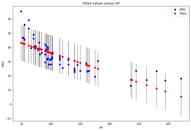
png
(b)
# Exactly the same exercise, but fit on a different response variable

Y = np.log(data['MPG']).rename('log MPG')
X = data[['HP']]
# Using manually coded solution
get_regression(X, Y)| coef | std err | t | P > |t| | |
|---|---|---|---|---|
| const | 4.013229 | 0.040124 | 100.021194 | 0.0 |
| HP | -0.004589 | 0.000309 | -14.873129 | 0.0 |
# Using statsmodels
results = sm.OLS(Y, sm.add_constant(X)).fit()
print(results.summary())
OLS Regression Results
==============================================================================
Dep. Variable: log MPG R-squared: 0.734
Model: OLS Adj. R-squared: 0.731
Method: Least Squares F-statistic: 221.2
Date: Sun, 15 Mar 2020 Prob (F-statistic): 9.62e-25
Time: 17:06:26 Log-Likelihood: 36.047
No. Observations: 82 AIC: -68.09
Df Residuals: 80 BIC: -63.28
Df Model: 1
Covariance Type: nonrobust
==============================================================================
coef std err t P>|t| [0.025 0.975]
------------------------------------------------------------------------------
const 4.0132 0.040 100.021 0.000 3.933 4.093
HP -0.0046 0.000 -14.873 0.000 -0.005 -0.004
==============================================================================
Omnibus: 4.454 Durbin-Watson: 1.026
Prob(Omnibus): 0.108 Jarque-Bera (JB): 3.827
Skew: 0.516 Prob(JB): 0.148
Kurtosis: 3.236 Cond. No. 299.
==============================================================================
Warnings:
[1] Standard Errors assume that the covariance matrix of the errors is correctly specified.# Plotting results
fig, ax = plt.subplots(figsize=(12, 8))
fig = sm.graphics.plot_fit(results, 1, ax=ax)
plt.show()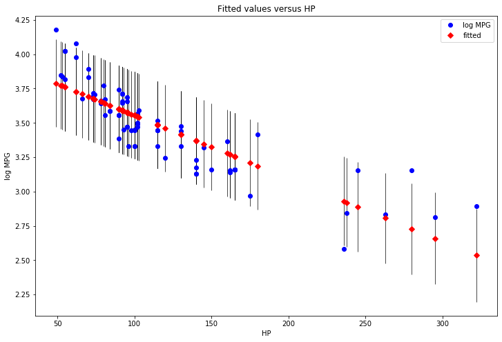
png
Exercise 14.9.7. Get the passenger car mileage data from
http://lib.stat.cmu.edu/DASL/Datafiles/carmpgdat.html
(a) Fit a multiple linear regression model to predict MPG (miles per gallon) from HP (horsepower). Summarize your analysis including a plot of the data with the fitted line.
(b) Use Mallow’s \(C_p\) to select a best sub-model. To search through all models try (i) all possible models, (ii) forward stepwise, (iii) backward stepwise. Summarize your findings.
(c) Repeat (b) but use BIC. Compare the results.
(d) Now use Lasso and compare the results.
Solution.
The exercise wording is unclear – if we specify that HP is the only covariate, the multiple linear regression and the simple linear regression are the same, and (a) is like the previous exercise.
We will elect to use VOL, HP, SP and WT as the covariates, and MPG as the response variable.
(a)
# Use full model

features = ['HP', 'SP', 'WT', 'VOL']

Y = data['MPG']
X = data[features]
# Using manually coded solution
get_regression(X, Y)| coef | std err | t | P > |t| | |
|---|---|---|---|---|
| const | 192.437753 | 23.531613 | 8.177839 | 3.351097e-12 |
| HP | 0.392212 | 0.081412 | 4.817602 | 6.671547e-06 |
| SP | -1.294818 | 0.244773 | -5.289864 | 1.019119e-06 |
| WT | -1.859804 | 0.213363 | -8.716617 | 2.888800e-13 |
| VOL | -0.015645 | 0.022825 | -0.685425 | 4.950327e-01 |
# Using statsmodels
results = sm.OLS(Y, sm.add_constant(X)).fit()
print(results.summary())
OLS Regression Results
==============================================================================
Dep. Variable: MPG R-squared: 0.873
Model: OLS Adj. R-squared: 0.867
Method: Least Squares F-statistic: 132.7
Date: Sun, 15 Mar 2020 Prob (F-statistic): 9.98e-34
Time: 17:06:27 Log-Likelihood: -220.00
No. Observations: 82 AIC: 450.0
Df Residuals: 77 BIC: 462.0
Df Model: 4
Covariance Type: nonrobust
==============================================================================
coef std err t P>|t| [0.025 0.975]
------------------------------------------------------------------------------
const 192.4378 23.532 8.178 0.000 145.580 239.295
HP 0.3922 0.081 4.818 0.000 0.230 0.554
SP -1.2948 0.245 -5.290 0.000 -1.782 -0.807
WT -1.8598 0.213 -8.717 0.000 -2.285 -1.435
VOL -0.0156 0.023 -0.685 0.495 -0.061 0.030
==============================================================================
Omnibus: 14.205 Durbin-Watson: 1.148
Prob(Omnibus): 0.001 Jarque-Bera (JB): 18.605
Skew: 0.784 Prob(JB): 9.12e-05
Kurtosis: 4.729 Cond. No. 1.16e+04
==============================================================================
Warnings:
[1] Standard Errors assume that the covariance matrix of the errors is correctly specified.
[2] The condition number is large, 1.16e+04. This might indicate that there are
strong multicollinearity or other numerical problems.# Plotting results
fig, ax = plt.subplots(figsize=(12, 8))
fig = sm.graphics.plot_fit(results, 1, ax=ax)
ax.set_ylabel("MPG")
ax.set_xlabel("HP")
ax.set_title("Linear Regression")
plt.show()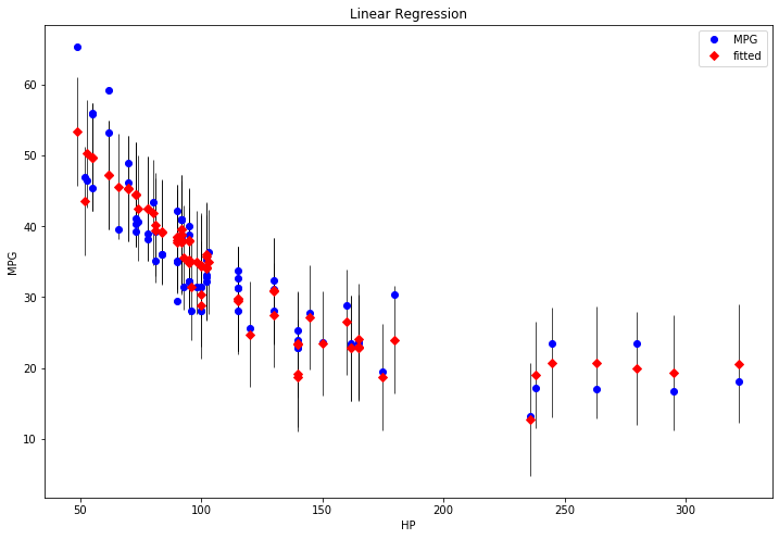
png
(b)
First, let’s create helper functions to calculate the model variance and Mallow’s \(C_p\):
def get_model_variance(X, Y):
    X = X.copy()

    # Create new column with all 1s for intercept at start
    X.insert(0, 'const', 1)

    # Least squares solution
    beta_hat = (np.linalg.inv(X.T @ X) @ X.T @ Y).to_numpy()

    # Predicted solutions
    Y_pred = X @ beta_hat

    # Prediction errors
    epsilon_hat = Y_pred - Y

    # Error on training data
    training_error = epsilon_hat.T @ epsilon_hat

    # Estimated error variance
    return (training_error / (Y.shape[0] - X.shape[1]))


def get_mallow_cp(X, Y, S, full_model_variance):
    if len(S) > 0:
        X = X[list(S)].copy()
        # Create new column with all 1s for intercept at start
        X.insert(0, 'const', 1)
    else:
        X = pd.DataFrame({'const': np.ones_like(Y)})

    # Least squares solution
    beta_hat = (np.linalg.inv(X.T @ X) @ X.T @ Y).to_numpy()

    # Predicted solutions
    Y_pred = X @ beta_hat

    # Prediction errors
    epsilon_hat = Y_pred - Y

    # Error on training data
    partial_training_error = epsilon_hat.T @ epsilon_hat

    # Increase size of S by to account for constant covariate
    return partial_training_error + 2 * (len(S) + 1) * full_model_variance
Next, let’s calculate and save the full model variance once, sine it’s used for every candidate model – and use it to define our custom score function.
full_model_variance = get_model_variance(X, Y)

def score_mallow_cp(S):
    return get_mallow_cp(X, Y, S, full_model_variance)
Finally, let’s do the submodel search.
First approach is an explicit search through all features:
# Recipe from itertools documentation, https://docs.python.org/2.7/library/itertools.html#recipes

from itertools import chain, combinations

def powerset(iterable):
    "powerset([1,2,3]) --> () (1,) (2,) (3,) (1,2) (1,3) (2,3) (1,2,3)"
    s = list(iterable)
    return chain.from_iterable(combinations(s, r) for r in range(len(s)+1))
# Iterate through the powerset and calculate the score for each value
results = [(S, score_mallow_cp(S)) for S in powerset(features)]
# Format as dataframe for ease of presentation
results = pd.DataFrame(results, columns=['S', 'score'])results| S | score | |
|---|---|---|
| 0 | () | 8134.147794 |
| 1 | (HP,) | 3102.805578 |
| 2 | (SP,) | 4318.234609 |
| 3 | (WT,) | 1519.372094 |
| 4 | (VOL,) | 7059.223052 |
| 5 | (HP, SP) | 2436.578842 |
| 6 | (HP, WT) | 1510.677511 |
| 7 | (HP, VOL) | 2354.823180 |
| 8 | (SP, WT) | 1463.076513 |
| 9 | (SP, VOL) | 3056.598857 |
| 10 | (WT, VOL) | 1542.174631 |
| 11 | (HP, SP, WT) | 1140.390871 |
| 12 | (HP, SP, VOL) | 2147.886521 |
| 13 | (HP, WT, VOL) | 1507.484328 |
| 14 | (SP, WT, VOL) | 1443.795004 |
| 15 | (HP, SP, WT, VOL) | 1160.807643 |
results[results.score == results.score.min()]| S | score | |
|---|---|---|
| 11 | (HP, SP, WT) | 1140.390871 |
This approach recommends the features HP, SP, and WT.
Next, let’s do forward stepwise feature selection:
current_subset = []
current_score = score_mallow_cp(current_subset)

while len(current_subset) < len(features):
    best_score, best_subset = current_score, current_subset
    updated = False
    for f in features:
        if f not in current_subset:
            candidate_subset = current_subset + [f]
            candidate_score = score_mallow_cp(candidate_subset)
            if candidate_score < best_score:
                best_score, best_subset = candidate_score, candidate_subset
                updated = True
    if not updated:
        break

    current_score, current_subset = best_score, best_subset

pd.DataFrame([[tuple(current_subset), current_score]], columns=['S', 'score'])| S | score | |
|---|---|---|
| 0 | (WT, SP, HP) | 1140.390871 |
This approach also recommends selecting these 3 features (order is irrelevant): WT, SP, HP
Finally, let’s so backward stepwise feature selection:
current_subset = features
current_score = score_mallow_cp(current_subset)

while len(current_subset) > 0:
    best_score, best_subset = current_score, current_subset
    updated = False
    for f in features:
        if f in current_subset:
            candidate_subset = [a for a in current_subset if a != f]
            candidate_score = score_mallow_cp(candidate_subset)
            if candidate_score < best_score:
                best_score, best_subset = candidate_score, candidate_subset
                updated = True
    if not updated:
        break

    current_score, current_subset = best_score, best_subset

pd.DataFrame([[tuple(current_subset), current_score]], columns=['S', 'score'])| S | score | |
|---|---|---|
| 0 | (HP, SP, WT) | 1140.390871 |
This approach also recommends selecting the same 3 features.
(c) This is analogous to (b), using the new scoring function.
Note that the book’s definition of BIC is:
\[ \text{BIC}(S) = \text{RSS}(S) + 2 |S| \hat{\sigma}^2 \]
while other sources apply a log to this quantity and scale it by the number of observations \(n\), e.g.
\[ \text{BIC} = n \log \left( \text{RSS} / n \right) + |S| \log n \]
We will use the later definition for this exercise.
def get_bic(X, Y, S):
    if len(S) > 0:
        X = X[list(S)].copy()
        # Create new column with all 1s for intercept at start
        X.insert(0, 'const', 1)
    else:
        X = pd.DataFrame({'const': np.ones_like(Y)})

    # Least squares solution
    beta_hat = (np.linalg.inv(X.T @ X) @ X.T @ Y).to_numpy()

    # Predicted solutions
    Y_pred = X @ beta_hat

    # Prediction errors
    epsilon_hat = Y_pred - Y

    # Error on training data
    rss = epsilon_hat.T @ epsilon_hat

    n = Y.shape[0]
    k = X.shape[1]

    return n * np.log(rss / n) + k * np.log(n)

def score_bic(S):
    return get_bic(X, Y, S)
Full search:
# Iterate through the powerset and calculate the score for each value
results = [(S, score_bic(S)) for S in powerset(features)]

# Format as dataframe for ease of presentation
results = pd.DataFrame(results, columns=['S', 'score'])results| S | score | |
|---|---|---|
| 0 | () | 381.100039 |
| 1 | (HP,) | 305.324815 |
| 2 | (SP,) | 332.832040 |
| 3 | (WT,) | 245.266568 |
| 4 | (VOL,) | 373.531556 |
| 5 | (HP, SP) | 288.594470 |
| 6 | (HP, WT) | 247.670065 |
| 7 | (HP, VOL) | 285.699095 |
| 8 | (SP, WT) | 244.895261 |
| 9 | (SP, VOL) | 307.747647 |
| 10 | (WT, VOL) | 249.455822 |
| 11 | (HP, SP, WT) | 225.425717 |
| 12 | (HP, SP, VOL) | 281.219751 |
| 13 | (HP, WT, VOL) | 250.346085 |
| 14 | (SP, WT, VOL) | 246.530268 |
| 15 | (HP, SP, WT, VOL) | 229.333642 |
results[results.score == results.score.min()]| S | score | |
|---|---|---|
| 11 | (HP, SP, WT) | 225.425717 |
Forward stepwise:
current_subset = []
current_score = score_bic(current_subset)

while len(current_subset) < len(features):
    best_score, best_subset = current_score, current_subset
    updated = False
    for f in features:
        if f not in current_subset:
            candidate_subset = current_subset + [f]
            candidate_score = score_bic(candidate_subset)
            if candidate_score < best_score:
                best_score, best_subset = candidate_score, candidate_subset
                updated = True
    if not updated:
        break

    current_score, current_subset = best_score, best_subset

pd.DataFrame([[tuple(current_subset), current_score]], columns=['S', 'score'])| S | score | |
|---|---|---|
| 0 | (WT, SP, HP) | 225.425717 |
Backward stepwise:
current_subset = features
current_score = score_bic(current_subset)

while len(current_subset) > 0:
    best_score, best_subset = current_score, current_subset
    updated = False
    for f in features:
        if f in current_subset:
            candidate_subset = [a for a in current_subset if a != f]
            candidate_score = score_bic(candidate_subset)
            if candidate_score < best_score:
                best_score, best_subset = candidate_score, candidate_subset
                updated = True
    if not updated:
        break

    current_score, current_subset = best_score, best_subset

pd.DataFrame([[tuple(current_subset), current_score]], columns=['S', 'score'])| S | score | |
|---|---|---|
| 0 | (HP, SP, WT) | 225.425717 |
All approaches recommend the same feature selection as the previous method – select the 3 features HP, SP, and WT.
(d) To use Lasso, we will need to minimize the L1 loss function for an arbitrary penalty parameter \(\lambda\):
\[ \sum_{i=1}^n (Y_i - \hat{Y}_i)^2 + \lambda \sum_{j=1}^k | \beta_j | \]
Since we are including a penalty parameter that affects both estimation and model selection, we will need to calculate this loss function on some test data distinct from the training data – the recommended approach being to use leave-one-out cross validation.
from scipy.optimize import minimize

# Lasso loss function
def lasso_loss(Y, Y_pred, beta, l1_penalty):
    error = Y - Y_pred
    return error.T @ error + l1_penalty * sum(abs(beta))

# Regularized fit
def fit_regularized(X, Y, l1_penalty):
    def loss_function(beta):
        return lasso_loss(Y, X @ beta, beta, l1_penalty)

    # Use the solution without penalties as an initial guess
    beta_initial_guess = (np.linalg.inv(X.T @ X) @ X.T @ Y).to_numpy()
    return minimize(loss_function, beta_initial_guess, method = 'Powell',
                    options={'xtol': 1e-8, 'disp': False, 'maxiter': 10000 })

# Leave-one-out cross-validation
def leave_one_out_cv_risk(X, Y, fitting_function):
    n = X.shape[1]
    total_risk = 0
    for i in range(n):
        XX = pd.concat([X.iloc[:i], X.iloc[i + 1:]])
        YY = pd.concat([Y.iloc[:i], Y.iloc[i + 1:]])
        beta = fitting_function(XX, YY).x
        validation_error = Y.iloc[i] - X.iloc[i] @ beta
        total_risk += validation_error * validation_error
    return total_risk / n

# Optimize over penalty parameter with best cross-validation risk
def optimize_l1_penalty(X, Y):
    def loss_function(l1_penalty_signed):
        # Ensure l1_penalty >= 0
        l1_penalty = abs(l1_penalty_signed)
        return leave_one_out_cv_risk(X, Y, lambda xx, yy: fit_regularized(xx, yy, l1_penalty))

    l1_penalty_initial_guess = 0.0
    return minimize(loss_function, l1_penalty_initial_guess, method = 'Powell',
                   options={'xtol': 1e-8, 'disp': True, 'maxiter': 10000 })
# Create a new dimension with constants, so the regressions have an intercept
X_c = X.copy()
X_c.insert(0, 'const', 1)# Optimize cross validation risk over penalties
best_penalty_res = optimize_l1_penalty(X_c, Y)
selected_l1_penalty = abs(best_penalty_res.x)
print("Selected penalty: ", selected_l1_penalty)Optimization terminated successfully.
Current function value: 61.554007
Iterations: 1
Function evaluations: 45
Selected penalty: 4.965056196086726e-07# Re-fit with selected penalty over the whole dataset
selected_fit = fit_regularized(X_c, Y, selected_l1_penalty)
beta = selected_fit.x
pd.DataFrame(beta.reshape(-1, 1), index=X_c.columns, columns=['coef'])| coef | |
|---|---|
| const | 192.437753 |
| HP | 0.392212 |
| SP | -1.294818 |
| WT | -1.859804 |
| VOL | -0.015645 |
The best leave-one-out cross validation for the Lasso procedure is achieved (according to our optimizer) at \(\lambda \approx\) 0, where all covariants have a non-zero coefficient (i.e. \(\beta_i \neq 0\) for all \(i\)).
In other words, Lasso with leave-one-out cross validation selects the full model.
Exercise 14.9.8. Assume that the errors are Normal. Show that the model with highest AIC is the model with lowest Mallows \(C_p\) statistic.
Mallows’ \(C_p\):
\[\hat{R}(S) = \hat{R}_\text{tr}(S) + 2 |S| \hat{\sigma}^2\]
AIC:
\[ \text{AIC} = \ell_S - |S|\]
Solution.
For the given definition, note that \(-2 \text{AIC} \hat{\sigma}^2 = -2 \ell_S \hat{\sigma}^2 + 2|S| \hat{\sigma}^2 = \hat{R}_\text{tr}(S) + 2 |S| \hat{\sigma}^2 = \hat{R}(S)\), given the log likelihood of a Normal model – so maximizing AIC is equivalent to minimizing Mallows \(C_p\).
Note that a more general result holds: rather than assuming the errors are Normal, one can assume that the distributions are part of a spherically symmetric family, i.e., modifying the distributions under an orthogonal transformation (and potentially removing invariance). See: Boisbunon, Aurélie, et al. “AIC, Cp and estimators of loss for elliptically symmetric distributions.” arXiv preprint arXiv:1308.2766 (2013).
Exercise 14.9.9. In this question we will take a closer look at the AIC method. Let \(X_1, \dots, X_n\) be iid observations. Consider two models \(\mathcal{M}_0\) and \(\mathcal{M}_1\). Under \(\mathcal{M}_0\) the data are assumed to be \(N(0, 1)\) while under \(M_1\) the data are assumed to be \(N(\theta, 1)\) for some unknown \(\theta \in \mathbb{R}\):
\[ \begin{align} \mathcal{M}_0 : X_1, \dots, X_n &\sim N(0, 1) \\ \mathcal{M}_1 : X_1, \dots, X_n &\sim N(\theta, 1), \; \theta \in \mathbb{R} \end{align} \]
This is just another way of viewing the hypothesis testing problem: \(H_0: \theta = 0\) versus \(H_1: \theta \neq 0\). Let \(\ell_n(\theta)\) be the log-likelihood function. The AIC score for a model is the log-likelihood at the MLE minus the number of parameters. (Some people multiply this score by 2 but that is irrelevant). Thus, the AIC score for \(\mathcal{M}_0\) is \(\text{AIC}_0 = \ell_n(0)\) and the AIC score for \(\mathcal{M}_1\) is \(\text{AIC}_1 = \ell_n(\hat{\theta}) - 1\). Suppose we choose the model with highest AIC score. Let \(J_n\) denote the selected model:
\[J_n = \begin{cases} 0 & \text{if } \text{AIC}_0 > \text{AIC}_1 \\ 1 & \text{if } \text{AIC}_1 > \text{AIC}_0 \end{cases}\]
(a) Suppose that \(\mathcal{M}_0\) is the true model, i.e. \(\theta = 0\). Find
\[ \lim_{n \rightarrow \infty} \mathbb{P}(J_n = 0) \]
Now compute \(\lim_{n \rightarrow \infty} \mathbb{P}(J_n = 0)\) when \(\theta \neq 0\).
(b) The fact that \(\lim_{n \rightarrow \infty} \mathbb{P}(J_n = 0) \neq 1\) when \(\theta = 0\) is why some people say that AIC “overfits.” But this is not quite true as we shall now see. Let \(\phi_\theta(x)\) denote a Normal density function with mean \(\theta\) and variance 1. Define
\[ \hat{f}_n(x) = \begin{cases} \phi_0(x) & \text{if } J_n = 0 \\ \phi_\overline{\theta}(x) & \text{if } J_n = 1 \end{cases}\]
If \(\theta = 0\), show that \(D(\phi_0, \hat{f}_n) \xrightarrow{\text{P}} 0\) as \(n \rightarrow \infty\) where
\[ D(f, g) = \int f(x) \log \left( \frac{f(x)}{g(x)} \right) dx \]
is the Kullback-Leibler distance. Show that \(D(\phi_\theta, \hat{f}_n) \xrightarrow{\text{P}} 0\) if \(\theta \neq 0\). Hence, AIC consistently estimates the true density even if it “overshoots” the correct model.
REMARK: If you are feeling ambitious, repeat the analysis for BIC which is the log-likelihood minus \((p / 2) \log n\) where \(p\) is the number of parameters and \(n\) is the sample size.
Solution.
(a) Note that the log-likelihood of the distribution \(N(\mu, \sigma^2)\) is:
\[ \begin{align} \ell_n(\mu, \sigma^2) &= \log \prod_{i=1}^n f(X_i | \mu, \sigma^2) \\ &= \sum_{i=1}^n \log f(X_i | \mu, \sigma^2) \\ &= - \frac{n}{2} \log 2\pi - \frac{n}{2} \log \sigma^2 - \frac{1}{2\sigma^2} \sum_{i=1}^n (X_i - \mu)^2 \end{align} \]
Then, we have:
\[ \begin{align} \mathbb{P}(J_n = 0) &= \mathbb{P}(\text{AIC}_0 > \text{AIC}_1) \\ &= \mathbb{P}(\ell_n(0) > \ell_n(\hat{\theta}) - 1) \\ &= \mathbb{P} \left(-\frac{n}{2} \log 2\pi - 0 - \frac{1}{2} \sum_{i=1}^n (X_i - 0)^2 > -\frac{n}{2} \log 2\pi - 0 - \frac{1}{2} \sum_{i=1}^n (X_i - \hat{\theta})^2 - 1 \right) \\ &= \mathbb{P}\left( -\frac{1}{2} \sum_{i=1}^n X_i^2 > -\frac{1}{2} \sum_{i=1}^n (X_i - \hat{\theta})^2 - 1\right) \\ &= \mathbb{P}\left( \sum_{i=1}^n \left((X_i - \hat{\theta})^2 - X_i^2 \right) > -2 \right) \\ &= \mathbb{P}\left( n \hat{\theta}^2 - 2 \hat{\theta} \sum_{i=1}^n X_i > -2 \right) \\ &= \mathbb{P}\left( n \overline{X}_n^2 - 2 \overline{X}_n n \overline{X}_n > -2\right) \\ &= \mathbb{P}\left( -n \overline{X}_n^2 > -2 \right) \\ &= \mathbb{P}\left(-\sqrt{\frac{2}{n}} < \overline{X}_n < \sqrt{\frac{2}{n}} \right) \end{align} \]
But \(X_i \sim N(\theta, 1)\), so \(n \overline{X}_n = \sum_i X_i \sim N(n\theta, n)\) and \(\overline{X}_n \sim N(\theta, 1/n)\). Then:
\[ \begin{align} \mathbb{P}(J_n = 0) &= \mathbb{P}\left(-\sqrt{\frac{2}{n}} < \overline{X}_n < \sqrt{\frac{2}{n}} \right) \\ &= \mathbb{P}\left(\frac{-\sqrt{\frac{2}{n}} - \theta}{\sqrt{1/n}} < \frac{\overline{X}_n - \theta}{\sqrt{1/n}} < \frac{\sqrt{\frac{2}{n}} - \theta}{\sqrt{1/n}} \right) \\ &= \mathbb{P}\left(-\sqrt{2} - \sqrt{n}\theta < Z < \sqrt{2} - \sqrt{n}\theta \right) \\ &= \Phi(\sqrt{2} - \sqrt{n}\theta) - \Phi(-\sqrt{2} - \sqrt{n}\theta) \end{align} \]
where \(\Phi\) is the CDF of the standard normal distribution \(N(0, 1)\).
When \(\theta = 0\),
\[\mathbb{P}(J_n = 0) = \Phi(\sqrt{2}) - \Phi(-\sqrt{2}) \approx 0.8427 \neq 0\]
When \(\theta \neq 0\),
\[\lim_{n \rightarrow \infty} \mathbb{P}(J_n = 0) = \lim_{n \rightarrow \infty}\Phi(\sqrt{2} - \sqrt{n}\theta) - \Phi(-\sqrt{2} - \sqrt{n}\theta) = \lim_{n \rightarrow \infty}\Phi(\sqrt{n}\theta) - \lim_{n \rightarrow \infty}\Phi(-\sqrt{n}\theta) = 0\]
(b) We have:
\[ D(\phi_\theta, \hat{f}_n) = \int \phi_\theta(x) \log \left(\frac{\phi_\theta(x)}{\hat{f}_n(x)} \right) dx = \int \left[\phi_\theta(x) \log \phi_\theta(x) - \phi_\theta(x) \log \hat{f}_n(x) \right] dx \]
But \(\lim_{n \rightarrow \infty} \hat{f}_n(x) = \phi_\theta(x)\), so the integrand goes to 0 at each x, and so \(D(\phi_\theta, \hat{f}_n) \xrightarrow{\text{P}} 0\).
REMARK: I am feeling ambitious. Let \(K_n\) denote the selected model:
\[ K_n = \begin{cases} 0 & \text{if } \text{BIC}_0 > \text{BIC}_1 \\ 1 & \text{if } \text{BIC}_1 > \text{BIC}_0 \end{cases}\]
where
\[ \text{BIC}_0 = \ell_n(0) \\ \text{BIC}_1 = \ell_n(\hat{\theta}) - \frac{1}{2} \log n \]
So,
\[ \begin{align} \mathbb{P}(K_n = 0) &= \mathbb{P}(\text{BIC}_0 > \text{BIC}_1) \\ &= \mathbb{P}\left(\ell_n(0) > \ell_n(\hat{\theta}) - \frac{1}{2} \log n \right) \\ &= \mathbb{P} \left(-\frac{n}{2} \log 2\pi - 0 - \frac{1}{2} \sum_{i=1}^n (X_i - 0)^2 > -\frac{n}{2} \log 2\pi - 0 - \frac{1}{2} \sum_{i=1}^n (X_i - \hat{\theta})^2 - \frac{1}{2} \log n \right) \\ &= \mathbb{P}\left( -\frac{1}{2} \sum_{i=1}^n X_i^2 > -\frac{1}{2} \sum_{i=1}^n (X_i - \hat{\theta})^2 - \frac{1}{2} \log n\right) \\ &= \mathbb{P}\left( \sum_{i=1}^n \left((X_i - \hat{\theta})^2 - X_i^2 \right) > -\log n \right) \\ &= \mathbb{P}\left( n \hat{\theta}^2 - 2 \hat{\theta} \sum_{i=1}^n X_i > -\log n \right) \\ &= \mathbb{P}\left( n \overline{X}_n^2 - 2 \overline{X}_n n \overline{X}_n > -\log n\right) \\ &= \mathbb{P}\left( -n \overline{X}_n^2 > -\log n \right) \\ &= \mathbb{P}\left(-\sqrt{\frac{\log n}{n}} < \overline{X}_n < \sqrt{\frac{\log n}{n}} \right) \\ &= \mathbb{P}\left(\frac{-\sqrt{\frac{\log n}{n}} - \theta}{\sqrt{1/n}} < \frac{\overline{X}_n - \theta}{\sqrt{1/n}} < \frac{\sqrt{\frac{\log n}{n}} - \theta}{\sqrt{1/n}} \right) \\ &= \mathbb{P}\left(-\sqrt{\log n} - \sqrt{n}\theta < Z < \sqrt{\log n} - \sqrt{n}\theta \right) \\ &= \Phi(\sqrt{\log n} - \sqrt{n}\theta) - \Phi(-\sqrt{\log n} - \sqrt{n}\theta) \end{align} \]
As \(O(\sqrt{log n}) < O(\sqrt{n})\), we get the result:
\[ \lim_{n \rightarrow \infty} \mathbb{P}(K_n = 0) = \begin{cases} 1 & \text{if } \theta = 0 \\ 0 & \text{if } \theta \neq 0 \end{cases}\]
Also, if we define:
\[\hat{g}_n(x) = \begin{cases} \phi_0(x) & \text{if } K_n = 0 \\ \phi_\overline{\theta}(x) & \text{if } K_n = 1 \end{cases}\]
then, again,
\[ D(\phi_\theta, \hat{g}_n) = \int \phi_\theta(x) \log \left(\frac{\phi_\theta(x)}{\hat{g}_n(x)} \right) dx = \int \left[\phi_\theta(x) \log \phi_\theta(x) - \phi_\theta(x) \log \hat{g}_n(x) \right] dx \]
But \(\lim_{n \rightarrow \infty} \hat{g}_n(x) = \phi_\theta(x)\), so the integrand goes to 0 at each x, and so \(D(\phi_\theta, \hat{g}_n) \xrightarrow{\text{P}} 0\).