- 10. Parametric Inference
- 10.1 Parameter of interest
- 10.2 The Method of Moments
- 10.3 Maximum Likelihood
- 10.4 Properties of Maximum Likelihood Estimators
- 10.5 Consistency of Maximum Likelihood Estimator
- 10.6 Equivalence of the MLE
- 10.7 Asymptotic Normality
- 10.8 Optimality
- 10.9 The Delta Method
- 10.10 Multiparameter Models
- 10.11 The Parametric Bootstrap
- 10.12 Technical Appendix
- 10.13 Exercises
- References
10. Parametric Inference
Parametric models are of the form
\[ \mathfrak{F} = \bigg\{ f(x; \theta) : \; \theta \in \Theta \bigg\} \]
where \(\Theta \subset \mathbb{R}^k\) is the parameter space and \(\theta = (\theta_1, \dots, \theta_k)\) is the parameter. The problem of inference then reduces to the problem of estimating parameter \(\theta\).
10.1 Parameter of interest
Often we are only interested in some function \(T(\theta)\). For example, if \(X \sim N(\mu, \sigma^2)\) then the parameter is \(\theta = (\mu, \sigma)\). If our goal is to estimate \(\mu\) then \(\mu = T(\theta)\) is called the parameter of interest and \(\sigma\) is called a nuisance parameter.
10.2 The Method of Moments
Suppose that the parameter \(\theta = (\theta_1, \dots, \theta_n)\) has \(k\) components. For \(1 \leq j \leq k\) define the \(j\)-th moment
\[ \alpha_j \equiv \alpha_j(\theta) = \mathbb{E}_\theta(X^j) = \int x^j dF_\theta(x)\]
and the \(j\)-th sample moment
\[ \hat{\alpha}_j = \frac{1}{n} \sum_{i=1}^n X_i^j \]
The method of moments estimator \(\hat{\theta}_n\) is defined to be the value of \(\theta\) such that
\[ \begin{align} \alpha_1(\hat{\theta}_n) &= \hat{\alpha_1} \\ \alpha_2(\hat{\theta}_n) &= \hat{\alpha_2} \\ \vdots \\ \alpha_k(\hat{\theta}_n) &= \hat{\alpha_k} \end{align} \]
This defines a system of \(k\) equations with \(k\) unknowns.
Theorem 10.6. Let \(\hat{\theta}_n\) denote the method of moments estimator. Under the conditions given in the appendix, the following statements hold:
The estimate \(\hat{\theta}_n\) exists with probability tending to 1.
The estimate is consistent: \(\hat{\theta}_n \xrightarrow{\text{P}} \theta\).
The estimate is asymptotically Normal:
\[\sqrt{n}(\hat{\theta}_n - \theta) \leadsto N(0, \Sigma) \]
where
\[ \Sigma = g \mathbb{E}_\theta (Y Y^T) g^T \\ Y = (X, X^2, \dots, X^k)^T, \quad g = (g_1, \dots, g_k) \quad \text{and} \quad g_j = \partial \alpha_j^{-1}(\theta)/\partial\theta \]
The last statement in Theorem 10.6 can be used to find standard errors and confidence intervals. However, there is an easier way: the bootstrap.
10.3 Maximum Likelihood
Let \(X_1, \dots, X_n\) be iid with PDF \(f(x; \theta)\).
The likelihood function is defined by
\[ \mathcal{L}_n(\theta) = \prod_{i=1}^n f(X_i; \theta) \]
The log-likelihood function is defined by \(\ell_n(\theta) = \log \mathcal{L}_n(\theta)\).
The likelihood function is just the joint density of the data, except we treat is as a function of parameter \(\theta\). Thus \(\mathcal{L}_n : \Theta \rightarrow [0, \infty)\). The likelihood function is not a density function; in general it is not true that \(\mathcal{L}_n\) integrates to 1.
The maximum likelihood estimator MLE, denoted by \(\hat{\theta}_n\), is the value of \(\theta\) that maximizes \(\mathcal{L}_n(\theta)\).
The maximum of \(\ell_n(\theta)\) occurs at the same place as the maximum of \(\mathcal{L}_n(\theta)\), so maximizing either leads to the same answer. Often it’s easier to maximize the log-likelihood.
%load_ext rpy2.ipython%%R
### Figure 9.2
n = 10
x = runif(n)
m = 100
par(mfrow=c(2,2),pty="s")
f = rep(0,m)
grid = seq(0,2,length=m)
f[grid < .75] = 1/.75
plot(grid,f,type="l",ylim=c(0,1.5),xlab="",ylab="",lwd=3,cex.lab=1.5)
points(x,rep(.5,n))
for(i in 1:n){
lines(c(x[i],x[i]),c(0,.5),lty=2,col=2)
}
f = rep(0,m)
grid = seq(0,2,length=m)
f[grid < 1] = 1
plot(grid,f,type="l",ylim=c(0,1.5),xlab="",ylab="",lwd=3,cex.lab=1.5)
points(x,rep(.5,n))
for(i in 1:n){
lines(c(x[i],x[i]),c(0,.5),lty=2,col=2)
}
f = rep(0,m)
grid = seq(0,2,length=m)
f[grid < 1.25] = 1/1.25
plot(grid,f,type="l",ylim=c(0,1.5),xlab="",ylab="",lwd=3,cex.lab=1.5)
points(x,rep(.5,n))
for(i in 1:n){
lines(c(x[i],x[i]),c(0,.5),lty=2,col=2)
}
theta = seq(.6,1.5,length=m)
lik = rep(0,m)
lik = 1/theta^n
lik[theta < max(x)] =0
plot(theta,lik,type="l",lwd=3,xlab="",ylab="",
cex.lab=1.5)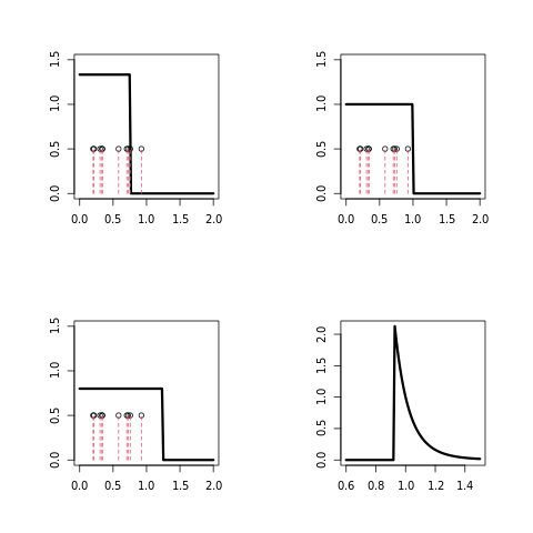
png
10.4 Properties of Maximum Likelihood Estimators
Under certain conditions on the model, the MLE \(\hat{\theta}_n\) possesses many properties that make it an appealing choice of estimator.
The main properties of the MLE are:
- It is consistent: \(\hat{\theta}_n \xrightarrow{\text{P}} \theta_*\), where \(\theta_*\) denotes the true value of parameter \(\theta\).
- It is equivariant: if \(\hat{\theta}_n\) is the MLE of \(\theta\) then \(g(\hat{\theta}_n)\) is the MLE of \(g(\theta)\).
- If is asymptotically Normal: \(\sqrt{n}(\hat{\theta} - \theta_*) / \hat{\text{se}} \leadsto N(0, 1)\) where \(\hat{\text{se}}\) can be computed analytically.
- It is asymptotically optimal or efficient: roughly, this means that among all well behaved estimators, the MLE has the smallest variance, at least for large samples.
- The MLE is approximately the Bayes estimator.
10.5 Consistency of Maximum Likelihood Estimator
If \(f\) and \(g\) are PDFs, define the Kullback-Leibler distance between \(f\) and \(g\) to be:
\[ D(f, g) = \int f(x) \log \left( \frac{f(x)}{g(x)} \right) dx \]
It can be shown that \(D(f, g) \geq 0\) and \(D(f, f) = 0\). For any \(\theta, \psi \in \Theta\) write \(D(\theta, \psi)\) to mean \(D(f(x; \theta), f(x; \psi))\). We will assume that \(\theta \neq \psi\) implies \(D(\theta, \psi) > 0\).
Let \(\theta_*\) denote the true value of \(\theta\). Maximizing \(\ell_n(\theta)\) is equivalent to maximizing
\[M_n(\theta) = \frac{1}{n} \sum_i \log \frac{f(X_i; \theta)}{f(X_i; \theta_*)}\]
By the law of large numbers, \(M_n(\theta)\) converges to:
\[ \begin{align} \mathbb{E}_{\theta_*} \left( \log \frac{f(X_i; \theta)}{f(X_i; \theta_*)} \right) & = \int \log \left( \frac{f(x; \theta)}{f(x; \theta_*)} \right) f(x; \theta_*) dx \\ & = - \int \log \left( \frac{f(x; \theta_*)}{f(x; \theta)} \right) f(x; \theta_*) dx \\ &= -D(\theta_*, \theta) \end{align} \]
Hence \(M_n(\theta) \approx -D(\theta_*, \theta)\) which is maximized at \(\theta_*\), since the KL distance is 0 when \(\theta_* = \theta\) and positive otherwise. Hence, we expect that the maximizer will tend to \(\theta_*\).
To prove this formally, we need more than \(M_n(\theta) \xrightarrow{\text{P}} -D(\theta_*, \theta)\). We need this convergence to be uniform over \(\theta\). We also have to make sure that the KL distance is well-behaved. Here are the formal details.
Theorem 10.13. Let \(\theta_*\) denote the true value of \(\theta\). Define
\[M_n(\theta) = \frac{1}{n} \sum_i \log \frac{f(X_i; \theta)}{f(X_i; \theta_*)}\]
and \(M(\theta) = -D(\theta_*, \theta)\). Suppose that
\[ \sup _{\theta \in \Theta} |M_n(\theta) - M(\theta)| \xrightarrow{\text{P}} 0 \]
and that, for every \(\epsilon > 0\),
\[ \sup _{\theta : |\theta - \theta_*| \geq \epsilon} M(\theta) < M(\theta_*)\]
Let \(\hat{\theta}_n\) denote the MLE. Then \(\hat{\theta}_n \xrightarrow{\text{P}} \theta_*\).
10.6 Equivalence of the MLE
Theorem 10.14. Let \(\tau = g(\theta)\) be a one-to-one function of \(\theta\). Let \(\hat{\theta}_n\) be the MLE of \(\theta\). Then \(\hat{\tau}_n = g(\hat{\theta}_n)\) is the MLE of \(\tau\).
Proof. Let \(h = g^{-1}\) denote the inverse of \(g\). Then \(\hat{\theta}_n = h(\hat{\tau}_n)\). For any \(\tau\), \(L(\tau) = \prod_i f(x_i; h(\tau)) = \prod_i f(x_i; \theta) = \mathcal{L}(\theta)\) where \(\theta = h(\tau)\). Hence, for any \(\tau\), \(\mathcal{L}_n(\tau) = \mathcal{L}(\theta) \leq \mathcal{L}(\hat{\theta}) = \mathcal{L}_n(\hat{\tau})\).
10.7 Asymptotic Normality
The score function is defined to be
\[ s(X; \theta) = \frac{\partial \log f(X; \theta)}{\partial \theta} \]
The Fisher information is defined to be
\[ \begin{align} I_n(\theta) &= \mathbb{V}_\theta \left( \sum_{i=1}^n s(X_i; \theta) \right) \\ &= \sum_{i=1}^n \mathbb{V}_\theta(s(X_i; \theta)) \end{align} \]
For \(n = 1\) we sometimes write \(I(\theta)\) instead of \(I_1(\theta)\).
It can be shown that \(\mathbb{E}_\theta(s(X; \theta)) = 0\). It then follows that \(\mathbb{V}_\theta(s(X; \theta)) = \mathbb{E}_\theta((s(X; \theta))^2)\). A further simplification of \(I_n(\theta)\) is given in the next result.
Note that \(\displaystyle 0\leq \mathcal{I}(\theta)\). A random variable carrying high Fisher information implies that the absolute value of the score is often high. The Fisher information is not a function of a particular observation, as the random variable X has been averaged out.
Theorem 10.17.
\[ I_n(\theta) = n I(\theta)\]
\[ \begin{align} I(\theta) & = \mathbb{E}_\theta \left( \frac{\partial \log f(X; \theta)}{\partial \theta} \right)^2 \\ &= \int \left( \frac{\partial \log f(x; \theta)}{\partial \theta} \right)^2 f(x; \theta) dx \end{align} \]
If \(\log f(x; \theta)\) is twice differentiable with respect to \(\theta\), and under certain regularity conditions, then the Fisher information may also be written as \[ \begin{align} I(\theta) & = -\mathbb{E}_\theta \left( \frac{\partial^2 \log f(X; \theta)}{\partial \theta^2} \right) \\ &= -\int \left( \frac{\partial^2 \log f(x; \theta)}{\partial \theta^2} \right) f(x; \theta) dx \end{align} \]
Theorem 10.18 (Asymptotic Normality of the MLE). Under appropriate regularity conditions, the following hold:
- Let \(\text{se} = \sqrt{1 / I_n(\theta)}\). Then,
\[ \frac{\hat{\theta}_n - \theta}{\text{se}} \leadsto N(0, 1) \]
- Let \(\hat{\text{se}} = \sqrt{1 / I_n(\hat{\theta}_n)}\). Then,
\[ \frac{\hat{\theta}_n - \theta}{\hat{\text{se}}} \leadsto N(0, 1) \]
The first statement says that \(\hat{\theta}_n \approx N(\theta, \text{se})\). The second statement says that this is still true if we replace the standard error \(\text{se}\) by its estimated standard error \(\hat{\text{se}}\).
Informally this says that the distribution of the MLE can be approximated with \(N(\theta, \hat{\text{se}})\). From this fact we can construct an asymptotic confidence interval.
Theorem 10.19. Let
\[ C_n = \left( \hat{\theta_n} - z_{\alpha/2} \hat{\text{se}}, \; \hat{\theta_n} + z_{\alpha/2} \hat{\text{se}} \right) \]
Then, \(\mathbb{P}_\theta(\theta \in C_n) \rightarrow 1 - \alpha\) as \(n \rightarrow \infty\).
Proof Let \(Z\) denote a standard random variable. Then,
\[ \begin{align} \mathbb{P}_\theta(\theta \in C_n) &= \mathbb{P}_\theta(\hat{\theta}_n - z_{\alpha/2} \hat{\text{se}} \leq \theta \leq \hat{\theta}_n + z_{\alpha/2} \hat{\text{se}}) \\ &= \mathbb{P}_\theta(-z_{\alpha/2} \leq \frac{\hat{\theta}_n - \theta}{\hat{\text{se}}} \leq z_{\alpha/2}) \\ &\rightarrow \mathbb{P}(-z_{\alpha/2} \leq Z \leq z_{\alpha/2}) = 1 - \alpha \end{align} \]
Let \(X\) be a Bernoulli trial. The Fisher information contained in \(X\) may be calculated to be \[ \begin{align} I(\theta) & = -\mathbb{E} \left( \frac{\partial^2 \log \left(\theta^X(1-\theta)^{(1-X)}\right)}{\partial \theta^2} \right) \\ &= -\mathbb{E} \left( \frac{\partial^2}{\partial \theta^2} \left[X\log \theta+(1-X)\log(1-\theta)\right] \right) \\ &=\mathbb{E}\left[\frac{X}{\theta^2}+\frac{1-X}{(1-\theta)^2}\right] \\ &=\frac{\theta}{\theta^2}+\frac{1-\theta}{(1-\theta)^2}\\ &=\frac{1}{\theta(1-\theta)}\\ \end{align} \]
Because Fisher information is additive, the Fisher information contained in \(n\) independent Bernoulli trials is therefore \[I(\theta)=\frac{n}{\theta(1-\theta)}\] Hence \[\hat{\text{se}}=\frac{1}{\sqrt{I_n(\hat{\theta})}}=\sqrt{\frac{\hat{\theta}(1-\hat{\theta})}{n}}\] An approximate 95% confidence inteval is \[\hat{\theta}_n\pm2\sqrt{\frac{\hat{\theta}(1-\hat{\theta})}{n}}\]
Let \(X\) be a Normal trial. The log-likelihood is \[\ell(\sigma)=-n\log\sigma-\frac{1}{2\sigma^2}\sum_{i=1}^{n}(x_i-\mu)^2\] Let \[\ell'(\sigma)=-n\frac{1}{\sigma}+\frac{1}{\sigma^3}\sum_{i=1}^{n}(x_i-\mu)^2=0\] get \[\hat{\sigma}=\sqrt{\frac{\sum_{i=1}^{n}(x_i-\mu)^2}{n}}\] To get the Fisher information , \[\log f(X;\sigma)=-\log\sigma-\frac{(X-\mu)^2}{2\sigma^2}\] with \[\frac{\partial^2\log f(X;\sigma)}{\partial^2\sigma}=\frac{1}{\sigma^2}-\frac{3(X-\mu)^2}{\sigma^4}\] and hence \[ \begin{align} I(\theta) & = -\mathbb{E} \left( \frac{1}{\sigma^2}-\frac{3(X-\mu)^2}{\sigma^4} \right) \\ &=-\frac{1}{\sigma^2}+\frac{3\sigma^2}{\sigma^4}\\ &=\frac{2}{\sigma^2} \end{align} \]
Hence \[\hat{\text{se}}=\frac{1}{\sqrt{I_n(\hat{\theta})}}=\frac{\hat{\sigma}_n}{\sqrt{2n}}\]
10.8 Optimality
Suppose that \(X_1, \dots, X_n \sim N(0, \sigma^2)\). The MLE is \(\hat{\theta}_n = \overline{X}_n\). Another reasonable estimator is the sample median \(\overline{\theta}_n\). The MLE satisfies
\[ \sqrt{n}(\hat{\theta}_n - \theta) \leadsto N(0, \sigma^2) \]
It can be proved that the median satisfies
\[ \sqrt{n}(\overline{\theta}_n - \theta) \leadsto N\left(0, \sigma^2 \frac{\pi}{2} \right) \]
This means that the median converges to the right value but has a larger variance than the MLE.
More generally, consider two estimators \(T_n\) and \(U_n\) and suppose that
\[ \sqrt{n}(T_n - \theta) \leadsto N(0, t^2) \quad \text{and} \quad \sqrt{n}(U_n - \theta) \leadsto N(0, u^2) \]
We define the asymptotic relative efficiency of U to T by \(ARE(U, T) = t^2/u^2\). In the Normal example, \(ARE(\overline{\theta}_n, \hat{\theta}_n) = 2 / \pi = 0.63\).
Theorem 10.23. If \(\hat{\theta}_n\) is the MLE and \(\widetilde{\theta}_n\) is any other estimator then
\[ ARE(\widetilde{\theta}_n, \hat{\theta}_n) \leq 1 \]
Thus, MLE has the smallest (asymptotic) variance and we say that MLE is efficient or asymptotically optimal.
The result is predicated over the model being correct – otherwise the MLE may no longer be optimal.
10.9 The Delta Method
Let \(\tau = g(\theta)\) where \(g\) is a smooth function. The maximum likelihood estimator of \(\tau\) is \(\hat{\tau} = g(\hat{\theta})\).
Theorem 10.24 (The Delta Method). If \(\tau = g(\theta)\) where \(g\) is differentiable and \(g'(\theta) \neq 0\) then
\[ \frac{\sqrt{n}(\hat{\tau}_n - \tau)}{\hat{\text{se}}(\hat{\tau})} \leadsto N(0, 1) \]
where \(\hat{\tau}_n = g(\hat{\theta})\) and
\[ \hat{\text{se}}(\hat{\tau}_n) = |g'(\hat{\theta})| \hat{\text{se}} (\hat{\theta}_n) \]
Hence, if
\[ C_n = \left( \hat{\tau}_n - z_{\alpha/2} \hat{\text{se}}(\hat{\tau}_n), \; \hat{\tau}_n + z_{\alpha/2} \hat{\text{se}}(\hat{\tau}_n) \right) \]
then \(\mathbb{P}_\theta(\tau \in C_n) \rightarrow 1 - \alpha\) as \(n \rightarrow \infty\).
10.10 Multiparameter Models
We can extend these ideas to models with several parameters.
Let \(\theta = (\theta_1, \dots, \theta_n)\) and let \(\hat{\theta} = (\hat{\theta}_1, \dots, \hat{\theta}_n)\) be the MLE. Let \(\ell_n = \sum_{i=1}^n \log f(X_i; \theta)\),
\[ H_{jj} = \frac{\partial^2 \ell_n}{\partial \theta_j^2} \quad \text{and} \quad H_{jk} = \frac{\partial^2 \ell_n}{\partial \theta_j \partial \theta_k} \]
Define the Fisher Information Matrix by
\[ I_n(\theta) = - \begin{bmatrix} \mathbb{E}_\theta(H_{11}) & \mathbb{E}_\theta(H_{12}) & \cdots & \mathbb{E}_\theta(H_{1k}) \\ \mathbb{E}_\theta(H_{21}) & \mathbb{E}_\theta(H_{22}) & \cdots & \mathbb{E}_\theta(H_{2k}) \\ \vdots & \vdots & \ddots & \vdots \\ \mathbb{E}_\theta(H_{k1}) & \mathbb{E}_\theta(H_{k2}) & \cdots & \mathbb{E}_\theta(H_{kk}) \end{bmatrix} \]
Let \(J_n(\theta) = I_n^{-1}(\theta)\) be the inverse of \(I_n\).
Theorem 10.27. Under appropriate regularity conditions,
\[ \sqrt{n}(\hat{\theta} - \theta) \approx N(0, J_n(\theta))\]
Also, if \(\hat{\theta}_j\) is the \(j\)-th component of \(\hat{\theta}\), then
\[ \frac{\sqrt{n}(\hat{\theta_j} - \theta_j)}{\hat{\text{se}}_j} \approx N(0, 1) \]
where \(\hat{\text{se}}_j^2\) is the \(j\)-th diagonal element of \(J_n\). The approximate covariance of \(\hat{\theta}_j\) and \(\hat{\theta}_k\) is \(\text{Cov}(\hat{\theta}_j, \hat{\theta}_k) \approx J_n(j, k)\).
There is also a multiparameter delta method. Let \(\tau = g(\theta_1, \dots, \theta_k)\) be a function and let
\[ \nabla g = \begin{pmatrix} \frac{\partial g}{\partial \theta_1} \\ \vdots \\ \frac{\partial g}{\partial \theta_k} \end{pmatrix} \]
be the gradient of \(g\).
Theorem 10.28 (Multiparameter delta method). Suppose that \(\nabla g\) evaluated at \(\hat{\theta}\) is not 0. Let \(\hat{\tau} = g(\hat{\theta})\). Then
\[ \frac{\sqrt{n}(\hat{\tau} - \tau)}{\hat{\text{se}}(\hat{\tau})} \leadsto N(0, 1) \]
where
\[ \hat{\text{se}}(\hat{\tau}) = \sqrt{\left(\hat{\nabla} g \right)^T \hat{J}_n \left(\hat{\nabla} g \right)} ,\]
\(\hat{J}_n = J_n(\hat{\theta}_n)\) and \(\hat{\nabla}g\) is \(\nabla g\) evaluated at \(\theta = \hat{\theta}\).
10.11 The Parametric Bootstrap
For parametric models, standard errors and confidence intervals may also be estimated using the bootstrap. There is only one change. In nonparametric bootstrap, we sampled \(X_1^*, \dots, X_n*\) from the empirical distribution \(\hat{F}_n\). In the parametric bootstrap we sample instead from \(f(x; \hat{\theta}_n)\). Here, \(\hat{\theta}_n\) could be the MLE or the method of moments estimator.
10.12 Technical Appendix
10.12.1 Proofs
Theorem 10.13. Let \(\theta_*\) denote the true value of \(\theta\). Define
\[M_n(\theta) = \frac{1}{n} \sum_i \log \frac{f(X_i; \theta)}{f(X_i; \theta_*)}\]
and \(M(\theta) = -D(\theta_*, \theta)\). Suppose that
\[ \sup _{\theta \in \Theta} |M_n(\theta) - M(\theta)| \xrightarrow{\text{P}} 0 \]
and that, for every \(\epsilon > 0\),
\[ \sup _{\theta : |\theta - \theta_*| \geq \epsilon} M(\theta) < M(\theta_*)\]
Let \(\hat{\theta}_n\) denote the MLE. Then \(\hat{\theta}_n \xrightarrow{\text{P}} \theta_*\).
Proof of Theorem 10.13. Since \(\hat{\theta}_n\) maximizes \(M_n(\theta)\), we have \(M_n(\hat{\theta}) \geq M_n(\theta_*)\). Hence,
\[ \begin{align} M(\theta_*) - M(\hat{\theta}_n) &= M_n(\theta_*) - M(\hat{\theta}_n) + M(\hat{\theta}_*) - M_n(\theta_*) \\ &\leq M_n(\hat{\theta}) - M(\hat{\theta}_n) + M(\theta_*) - M_n(\theta_*) \\ &\leq \sup_\theta | M_n(\theta) - M(\theta) | + M(\theta_*) - M_n(\theta_*) \\ &\xrightarrow{\text{P}} 0 \end{align} \]
It follows that, for any \(\delta > 0\),
\[\mathbb{P}(M(\hat{\theta}_n) < M(\theta_*) - \delta) \rightarrow 0\]
Pick any \(\epsilon > 0\). There exists \(\delta > 0\) such that \(|\theta - \theta_*| \geq \epsilon\) implies that \(M(\theta) < M(\theta_*) - \delta\). Hence,
\[\mathbb{P}(|\hat{\theta}_n - \theta_*| > \epsilon) \leq \mathbb{P}\left( M(\hat{\theta}_n) < M(\theta_*) - \delta \right) \rightarrow 0\]
Lemma 10.31. The score function satisfies
\[\mathbb{E}[s(X; \theta)] = 0\]
Proof. Note that \(1 = \int f(x; \theta) dx\). Differentiate both sides of this equation to get
\[ \begin{align} 0 &= \frac{\partial}{\partial \theta} \int f(x; \theta)dx = \int \frac{\partial}{\partial \theta} f(x; \theta) dx \\ &= \int \frac{\frac{\partial f(x; \theta)}{\partial \theta}}{f(x; \theta)} f(x; \theta) dx = \int \frac{\partial \log f(x; \theta)}{\partial \theta} f(x; \theta) dx \\ &= \int s(x; \theta) f(x; \theta) dx = \mathbb{E}[s(X; \theta)] \end{align} \]
Theorem 10.18 (Asymptotic Normality of the MLE). Under appropriate regularity conditions, the following hold:
- Let \(\text{se} = \sqrt{1 / I_n(\theta)}\). Then,
\[ \frac{\hat{\theta}_n - \theta}{\text{se}} \leadsto N(0, 1) \]
- Let \(\hat{\text{se}} = \sqrt{1 / I_n(\hat{\theta}_n)}\). Then,
\[ \frac{\hat{\theta}_n - \theta}{\hat{\text{se}}} \leadsto N(0, 1) \]
Proof of Theorem 10.18. Let \(\ell(\theta) = \log \mathcal{L}(\theta)\). Then
\[0 = \ell'(\hat{\theta}) \approx \ell'(\theta) + (\hat{\theta} - \theta) \ell''(\theta)\]
Rearrange the above equation to get \(\hat{\theta} - \theta = -\ell'(\theta) / \ell''(\theta)\), or
\[ \sqrt{n}(\hat{\theta} - \theta) = \frac{\frac{1}{\sqrt{n}}\ell'(\theta)}{-\frac{1}{n}\ell''(\theta)} = \frac{\text{TOP}}{\text{BOTTOM}}\]
Let \(Y_i = \partial \log f(X_i, \theta) / \partial \theta\). From the previous lemma \(\mathbb{E}(Y_i) = 0\) and also \(\mathbb{V}(Y_i) = I(\theta)\). Hence,
\[\text{TOP} = n^{-1/2} \sum_i Y_i = \sqrt{n} \overline{Y} = \sqrt{n} (\overline{Y} - 0) \leadsto W \sim N(0, I)\]
by the central limit theorem. Let \(A_i = -\partial^2 \log f(X_i; \theta) / \partial theta^2\). Then \(\mathbb{E}(A_i) = I(\theta)\) and
\[\text{BOTTOM} = \overline{A} \xrightarrow{\text{P}} I(\theta)\]
by the law of large numbers. Apply Theorem 6.5 part (e) to conclude that
\[\sqrt{n}(\hat{\theta} - \theta) \leadsto \frac{W}{I(\theta)} \sim N \left(0, \frac{1}{I(\theta)} \right)\]
Assuming that \(I(\theta)\) is a continuous function of \(\theta\), it follows that \(I(\hat{\theta}_n) \xrightarrow{\text{P}} I(\theta)\). Now
\[ \begin{align} \frac{\hat{\theta}_n - \theta}{\hat{\text{se}}}&= \sqrt{n} I^{1/2}(\hat{\theta_n})(\hat{\theta_n} - \theta) \\ &= \left\{ \sqrt{n} I^{1/2}(\theta)(\hat{\theta}_n - \theta)\right\} \left\{ \frac{I(\hat{\theta}_n)}{I(\theta)} \right\}^{1/2} \end{align} \]
The first term tends in distribution to \(N(0, 1)\). The second term tends in probability to 1. The result follows from Theorem 6.5 part (e).
Theorem 10.24 (The Delta Method). If \(\tau = g(\theta)\) where \(g\) is differentiable and \(g'(\theta) \neq 0\) then
\[ \frac{\sqrt{n}(\hat{\tau}_n - \tau)}{\hat{\text{se}}(\hat{\tau})} \leadsto N(0, 1) \]
where \(\hat{\tau}_n = g(\hat{\theta})\) and
\[ \hat{\text{se}}(\hat{\tau}_n) = |g'(\hat{\theta})| \hat{\text{se}} (\hat{\theta}_n) \]
Hence, if
\[ C_n = \left( \hat{\tau}_n - z_{\alpha/2} \hat{\text{se}}(\hat{\tau}_n), \; \hat{\tau}_n + z_{\alpha/2} \hat{\text{se}}(\hat{\tau}_n) \right) \]
then \(\mathbb{P}_\theta(\tau \in C_n) \rightarrow 1 - \alpha\) as \(n \rightarrow \infty\).
Outline of proof of Theorem 10.24. Write,
\[\hat{\tau} = g(\hat{\theta}) \approx g(\theta) + (\hat{\theta} - \theta)g'(\theta) = \tau + (\hat{\theta} - \theta)g'(\theta)\]
Thus,
\[\sqrt{n}(\hat{\tau} - \tau) \approx \sqrt{n}(\hat{\theta} - \theta)g'(\theta)\]
and hence
\[\frac{\sqrt{n}I^{1/2}(\theta)(\hat{\theta} - \theta)}{g'(\theta)} \approx \sqrt{n}I^{1/2}(\theta)(\hat{\theta} - \theta)\]
Theorem 10.18 tells us that the right hand side tends in distribution to \(N(0, 1)\), hence
\[\frac{\sqrt{n}I^{1/2}(\theta)(\hat{\theta} - \theta)}{g'(\theta)} \leadsto N(0, 1)\]
or, in other words,
\[\hat{\tau} \approx N(\tau, \text{se}^2(\hat{\tau}_n))\]
where
\[\text{se}^2(\hat{\tau}_n) = \frac{(g'(\theta))^2}{nI(\theta)}\]
The result remains true if we substitute \(\hat{\theta}\) for \(\theta\) by Theorem 6.5 part (e).
10.12.2 Sufficiency
A statistic is a function \(T(X^n)\) of the data. A sufficient statistic is a statistic that contains all of the information in the data.
Write \(x^n \leftrightarrow y^n\) if \(f(x^n; \theta) = c f(y^n; \theta)\) for some constant \(c\) that might depend on \(x^n\) and \(y^n\) but not \(\theta\). A statistic is sufficient if \(T(x^n) \leftrightarrow T(y^n)\) implies that \(x^n \leftrightarrow y^n\).
Notice that if \(x^n \leftrightarrow y^n\) then the likelihood functions based on \(x^n\) and \(y^n\) have the same shape. Roughly speaking, a statistic is sufficient if we can calculate the likelihood function knowing only \(T(X^n)\).
A statistic \(T\) is minimally sufficient if it is sufficient and it is a function of every other sufficient statistic.
Theorem 10.36. \(T\) is minimally sufficient if \(T(x^n) = T(y^n)\) if and only if \(x^n \leftrightarrow y^n\).
The usual definition of sufficiency is this: \(T\) is sufficient if the distribution of \(X^n\) given \(T(X^n) = t\) does not depend on \(\theta\).
Theorem 10.40 (Factorization Theorem). \(T\) is sufficient if and only if there are functions \(g(t, \theta)\) and \(h(x)\) such that \(f(x^n; \theta) = g(t(x^n); \theta)h(x^n)\).
Theorem 10.42 (Rao-Blackwell). Let \(\hat{\theta}\) be an estimator and let \(T\) be a sufficient statistic. Define a new estimator by
\[\overline{\theta} = \mathbb{E}(\hat{\theta} | T)\]
Then, for every \(\theta\),
\[R(\theta, \overline{\theta}) \leq R(\theta, \hat{\theta})\]
where \(R(\theta, \hat{\theta}) = \mathbb{E}_\theta[(\theta - \hat{\theta})^2]\) denote the MSE of an estimator.
10.12.3 Exponential Families
We say that \(\{f(x; \theta) : \theta \in \Theta\}\) is a one-parameter exponential family if there are functions \(\eta(\theta)\), \(B(\theta)\), \(T(x)\) and \(h(x)\) such that
\[f(x; \theta) = h(x) e^{\eta(\theta)T(x) - B(\theta)}\]
It is easy to see that \(T(X)\) is sufficient. We call \(T\) the natural sufficient statistic.
We can rewrite an exponential family as
\[f(x; \eta) = h(x) e^{\eta T(x) - A(\eta)}\]
where \(\eta = \eta(\theta)\) is called the natural parameter and
\[A(\eta) = \log \int h(x) e^{\eta T(x)} dx\]
Let \(X_1, \dots, X_n\) be iid from an exponential family. Then \(f(x^n; \theta)\) is an exponential family:
\[f(x^n; \theta) = h_n(x^n) e^{\eta(\theta) T_n(x^n) - B_n(\theta)}\]
where \(h_n(x^n) = \prod_i h(x_i)\), \(T_n(x^n) = \sum_i T(x_i)\) and \(B_n(\theta) = nB(\theta)\). This implies that \(\sum_i T(X_i)\) is sufficient.
Theorem 10.47. Let \(X\) have an exponential family. Then,
\[ \mathbb{E}(T(X)) = A'(\eta), \quad \mathbb{V}(T(X)) = A''(\eta) \]
If \(\theta = (\theta_1, \dots, \theta_n)\) is a vector, then we say that \(f(x; \theta)\) has exponential family form if
\[ f(x; \theta) = h(x) \exp \left\{ \sum_{j=1}^k \eta_j(\theta) T_j(x) - B(\theta) \right\}\]
Again, \(T = (T_1, \dots, T_k)\) is sufficient and \(n\) iid samples also has exponential form with sufficient statistic \(\left(\sum_i T_1(X_i), \dots, \sum_i T_k(X_i)\right)\).
10.13 Exercises
Exercise 10.13.1. Let \(X_1, \dots, X_n \sim \text{Gamma}(\alpha, \beta)\). Find the method of moments estimator for \(\alpha\) and \(\beta\).
Solution.
Let \(X \sim \text{Gamma}(\alpha, \beta)\). The PDF is
\[ f_X(x) = \frac{\beta^\alpha}{\Gamma(\alpha)} x^{\alpha - 1} e^{-\beta x} \quad \text{for } x > 0 \]
We have:
\[ \begin{align} \mathbb{E}(X) &= \int x f_X(x) dx \\ &= \int_0^\infty x \frac{\beta^\alpha}{\Gamma(\alpha)} x^{\alpha - 1} e^{-\beta x} dx \\ &= \frac{\alpha}{\beta} \int_0^\infty\frac{\beta^{\alpha + 1}}{\Gamma(\alpha + 1)} x^\alpha e^{-\beta x} dx \\ &= \frac{\alpha}{\beta} \end{align} \] We also have:
\[ \begin{align} \mathbb{E}(X^2) &= \int x^2 f_X(x) dx \\ &= \int_0^\infty x^2 \frac{\beta^\alpha}{\Gamma(\alpha)} x^{\alpha - 1} e^{-\beta x} dx \\ &= \frac{\alpha (\alpha + 1)}{\beta^2} \int_0^\infty\frac{\beta^{\alpha + 2}}{\Gamma(\alpha + 2)} x^{\alpha + 1} e^{-\beta x} dx \\ &= \frac{\alpha (\alpha + 1)}{\beta^2} \end{align} \] Therefore,
\[ \mathbb{V}(X) = \mathbb{E}(X^2) - \mathbb{E}(X)^2 = \frac{\alpha (\alpha + 1)}{\beta^2} - \frac{\alpha^2}{\beta^2} = \frac{\alpha}{\beta^2} \]
The first two moments are:
\[ \alpha_1 = \mathbb{E}(X) = \frac{\alpha}{\beta}\\ \alpha_2 = \mathbb{E}(X^2) = \mathbb{V}(X) + \mathbb{E}(X)^2 = \frac{\alpha}{\beta^2} + \frac{\alpha^2}{\beta^2} = \frac{\alpha(\alpha + 1)}{\beta^2} \]
We have the sample moments:
\[\hat{\alpha}_1 = \frac{1}{n}\sum_{i=1}^n X_i \quad \quad \hat{\alpha}_2 = \frac{1}{n}\sum_{i=1}^n X_i^2\]
Equating these we get:
\[ \hat{\alpha}_1 = \frac{\hat{\alpha}_n}{\hat{\beta}_n} \quad \quad \hat{\alpha}_2 = \frac{\hat{\alpha}_n(\hat{\alpha}_n + 1)}{\hat{\beta}_n^2} \]
Solving these we get the method of moments estimators for \(\alpha\) and \(\beta\):
\[ \hat{\alpha}_n = \frac{\hat{\alpha}_1^2}{\hat{\alpha}_2 - \hat{\alpha}_1^2} \quad \quad \hat{\beta}_n = \frac{\hat{\alpha}_1}{\hat{\alpha}_2 - \hat{\alpha}_1^2} \]
Exercise 10.13.2. Let \(X_1, \dots, X_n \sim \text{Uniform}(a, b)\) where \(a, b\) are unknown parameters and \(a < b\).
(a) Find the method of moments estimators for \(a\) and \(b\).
(b) Find the MLE \(\hat{a}\) and \(\hat{b}\).
(c) Let \(\tau = \int x dF(x)\). Find the MLE of \(\tau\).
(d) Let \(\hat{\tau}\) be the MLE from the previous item. Let \(\tilde{\tau}\) be the nonparametric plug-in estimator of \(\tau = \int x dF(x)\). Suppose that \(a = 1\), \(b = 3\) and \(n = 10\). Find the MSE of \(\hat{\tau}\) by simulation. Find the MSE of \(\tilde{\tau}\) analytically. Compare.
Solution.
(a)
Let \(X \sim \text{Uniform}(a, b)\). Then:
- \[\mathbb{E}(X) = \int_a^b x \frac{1}{b - a} dx = \frac{a + b}{2}\]
- \[\mathbb{E}(X^2) = \int_a^b x^2 \frac{1}{b - a} dx = \frac{a^2 + ab + b^2}{3}\]
- \[\mathbb{V}(X) = \mathbb{E}(X^2) - \mathbb{E}(X)^2 = \frac{a^2 + ab + b^2}{3} - \frac{a^2 + 2ab + b^2}{4} = \frac{(b - a)^2}{12}\] The first two moments are:
\[ \alpha_1 = \mathbb{E}(X) = \frac{a + b}{2} \\ \alpha_2 = \mathbb{E}(X^2) = \mathbb{V}(X) + \mathbb{E}(X)^2 = \frac{(b - a)^2}{12} + \frac{(a + b)^2}{4} = \frac{a^2 + ab + b^2}{3} \]
We have the sample moments:
\[\hat{\alpha}_1 = \frac{1}{n}\sum_{i=1}^n X_i \quad \quad \hat{\alpha}_2 = \frac{1}{n}\sum_{i=1}^n X_i^2\]
Equating these we get:
\[ \hat{\alpha}_1 = \frac{\hat{a} + \hat{b}}{2} \quad \quad \hat{\alpha}_2 = \frac{(\hat{b} - \hat{a})^2}{12} + \frac{(\hat{a} + \hat{b})^2}{4} \]
Solving these we get the method of moment estimators for \(a\) and \(b\):
\[ \hat{a} = \hat{\alpha}_1 - \sqrt{3}(\hat{\alpha}_1^2 - \hat{\alpha}_2) \quad \quad \hat{b} = \hat{\alpha}_1 + \sqrt{3}(\hat{\alpha}_1^2 - \hat{\alpha}_2) \]
(b)
The probability density function for each \(X_i\) is
\[f(x; (a, b)) = \begin{cases} (b - a)^{-1} & \text{if } a \leq x \leq b \\ 0 & \text{otherwise} \end{cases}\]
The likelihood function is
\[\mathcal{L}_n(a, b) = \prod_{i=1}^n f(X_i; (a, b)) = \begin{cases} (b-a)^{-n} & \text{if } a \leq X_i \leq b \text{ for all } X_i\\ 0 & \text{otherwise} \end{cases} \]
The parameters that maximize the likelihood function make the \(b - a\) as small as possible – that is, we should pick the maximum \(a\) and the minimum \(b\) for which the likelihood function is non-zero. So the MLEs are:
\[\hat{a} = \min \{X_1, \dots, X_n \} \quad \quad \hat{b} = \max \{X_1, \dots, X_n \}\]
(c)
\(\tau = \int x dF(x) = \mathbb{E}(x) = (a + b)/2\), so since the MLE is equivariant, the MLE of \(\tau\) is
\[\hat{\tau} = \frac{\hat{a} + \hat{b}}{2} = \frac{\min \{X_1, \dots, X_n\} + \max\{X_1, \dots, X_n\}}{2}\]
(d)
import numpy as np

a = 1
b = 3
n = 10

X = np.random.uniform(low=a, high=b, size=n)
tau_hat = (X.min() + X.max()) / 2
# Nonparametric bootstrap to find MSE of tau_hat
B = 10000
t_boot = np.empty(B)
for i in range(B):
xx = np.random.choice(X, n, replace=True)
t_boot[i] = (xx.min() + xx.max()) / 2
se = t_boot.std()
print("MSE for tau_hat: \t %.3f" % se)MSE for tau_hat: 0.091Analytically, we have:
\[ \begin{align} \mathbb{V}(\tilde{\tau}) &= \mathbb{E}(\tilde{\tau}^2) - (\mathbb{E}(\tilde{\tau}))^2 \\ &= \frac{1}{n^2}\left(\mathbb{E}\left[ \left(\sum_{i=1}^n X_i\right)^2\right] - \left(\mathbb{E}\left[\sum_{i=1}^n X_i \right]\right)^2\right) \\ &= \frac{1}{n^2}\left( \mathbb{E}\left[ \sum_{i=1}^n X_i^2 + \sum_{i=1}^n \sum_{j=1, j \neq i}^n X_i X_j \right] - \left(n \frac{a + b}{2}\right)^2\right) \\ &= \frac{1}{n^2}\left( \sum_{i=1}^n \mathbb{E}[X_i^2] + \sum_{i=1}^n \sum_{j=1, j \neq i}^n \mathbb{E}[X_i]\mathbb{E}[X_j] - \left(n \frac{a + b}{2}\right)^2\right) \\ &= \frac{1}{n^2}\left( n \frac{a^2 + ab + b^2}{3} + n(n-1) \left(\frac{a+b}{2}\right)^2 - n^2\left(\frac{a + b}{2}\right)^2\right) \\ &= \frac{1}{n^2}\left( n \frac{a^2 + ab + b^2}{3} - n \left(\frac{a+b}{2}\right)^2 \right) \\ &= \frac{1}{n} \left( \frac{a^2 + ab + b^2}{3} - \frac{a^2 + 2ab + b^2}{4}\right) \\ &= \frac{1}{n} \frac{(b - a)^2}{12} \end{align} \]
Therefore,
\[\text{se}(\tilde{\tau}) = \sqrt{\frac{1}{n} \frac{(b - a)^2}{12}}\]
se_tau_tilde = np.sqrt((1/n) * ((b - a)**2 / 12))

print("MSE for tau_tilde: \t %.3f" % se_tau_tilde)
MSE for tau_tilde: 0.183Exercise 10.13.3. Let \(X_1, \dots, X_n \sim N(\mu, \sigma^2)\). Let \(\tau\) be the 0.95 percentile, i.e. \(\mathbb{P}(X < \tau) = 0.95\).
(a) Find the MLE of \(\tau\).
(b) Find an expression for an approximate \(1 - \alpha\) confidence interval for \(\tau\).
(c) Suppose the data are:
\[ \begin{matrix} 3.23 & -2.50 & 1.88 & -0.68 & 4.43 & 0.17 \\ 1.03 & -0.07 & -0.01 & 0.76 & 1.76 & 3.18 \\ 0.33 & -0.31 & 0.30 & -0.61 & 1.52 & 5.43 \\ 1.54 & 2.28 & 0.42 & 2.33 & -1.03 & 4.00 \\ 0.39 \end{matrix} \]
Find the MLE \(\hat{\tau}\). Find the standard error using the delta method. Find the standard error using the parametric bootstrap.
Solution.
(a)
Let \(Z \sim N(0, 1)\), so \((X - \mu) / \sigma \sim Z\). We have:
\[ \begin{align} \mathbb{P}(X < \tau) &= 0.95 \\ \mathbb{P}\left(\frac{X - \mu}{\sigma} < \frac{\tau - \mu}{\sigma}\right) &= 0.95 \\ \mathbb{P}\left(Z < \frac{\tau - \mu}{\sigma}\right) &= 0.95 \\ \frac{\tau - \mu}{\sigma} &= z_{5\%} \\ \tau &= \mu + z_{5\%} \sigma \end{align} \]
Since the MLE is equivariant, \(\hat{\tau} = \hat{\mu} + z_{5\%} \hat{\sigma}\), where \(\hat{\mu}, \hat{\sigma}\) are the MLEs for the Normal distribution parameters:
\[ \hat{\mu} = n^{-1} \sum_{i=1}^n X_i \quad \quad \hat{\sigma} = \sqrt{n^{-1} \sum_{i=1}^n (X_i - \overline{X})^2} \]
(b)
Let’s use the multiparameter delta method.
We have \(\tau = g(\mu, \sigma) = \mu + z_{5\%} \sigma\), so
\[ \nabla g = \begin{bmatrix} \partial g / \partial \mu \\ \partial g / \partial \sigma \end{bmatrix} = \begin{bmatrix} 1 \\ z_{5\%} \end{bmatrix}\].
Let \(X\) be a Normal trial. The log-likelihood is \[\ell(\sigma)=-n\log\sigma-\frac{1}{2\sigma^2}\sum_{i=1}^{n}(x_i-\mu)^2\] Let \[\ell'(\sigma)=-n\frac{1}{\sigma}+\frac{1}{\sigma^3}\sum_{i=1}^{n}(x_i-\mu)^2=0\] get \[\hat{\sigma}=\sqrt{\frac{\sum_{i=1}^{n}(x_i-\mu)^2}{n}}\] To get the Fisher information , \[\log f(X;\sigma)=-\log\sigma-\frac{(X-\mu)^2}{2\sigma^2}\] with \[\frac{\partial^2\log f(X;\sigma)}{\partial^2\sigma}=\frac{1}{\sigma^2}-\frac{3(X-\mu)^2}{\sigma^4}\] and hence
\[I(\mu)=\frac{1}{\sigma^2}\] \[ \begin{align} I(\sigma) & = -\mathbb{E} \left( \frac{1}{\sigma^2}-\frac{3(X-\mu)^2}{\sigma^4} \right) \\ &=-\frac{1}{\sigma^2}+\frac{3\sigma^2}{\sigma^4}\\ &=\frac{2}{\sigma^2} \end{align} \] The Fisher Information Matrix for the Normal process is
\[ I_n(\mu, \sigma) = \begin{bmatrix} n / \sigma^2 & 0 \\ 0 & 2n / \sigma^2 \end{bmatrix} \]
then its inverse is
\[ J_n = I_n^{-1}(\mu, \sigma) = \frac{1}{n} \begin{bmatrix} \sigma^2 & 0 \\ 0 & \sigma^2/2 \end{bmatrix} \]
and the standard error estimate for our new parameter variable is
\[\hat{\text{se}}(\hat{\tau}) = \sqrt{(\hat{\nabla} g)^T \hat{J}_n (\hat{\nabla} g)} = \hat{\sigma} \sqrt{n^{-1}(1 + z_{5\%}^2 / 2)}\]
A \(1 - \alpha\) confidence interval for \(\hat{\tau}\), then, is
\[ C_n = \left( \hat{\mu} + \hat{\sigma}\left( z_{5\%} - z_{\alpha / 2} \sqrt{n^{-1}(1 + z_{5\%}^2 / 2)} \right), \; \hat{\mu} + \hat{\sigma}\left( z_{5\%} + z_{\alpha / 2} \sqrt{n^{-1}(1 + z_{5\%}^2 / 2)} \right) \right) \]
(c)
import numpy as np
from scipy.stats import norm

z_05 = norm.ppf(0.95)
z_025 = norm.ppf(0.975)
X = np.array([
3.23, -2.50, 1.88, -0.68, 4.43, 0.17,
1.03, -0.07, -0.01, 0.76, 1.76, 3.18,
0.33, -0.31, 0.30, -0.61, 1.52, 5.43,
1.54, 2.28, 0.42, 2.33, -1.03, 4.00,
0.39
])# Estimate the MLE tau_hat
n = len(X)
mu_hat = X.mean()
sigma_hat = X.std()
tau_hat = mu_hat + z_05 * sigma_hat
print("Estimated tau: %.3f" % tau_hat)Estimated tau: 4.180# Confidence interval using delta method
se_tau_hat = sigma_hat * np.sqrt((1/n) * (1 + z_05 * z_05 / 2))
confidence_interval = (tau_hat - z_025 * se_tau_hat, tau_hat + z_025 * se_tau_hat)
print("Estimated tau (delta method, 95%% confidence interval): \t (%.3f, %.3f)" % confidence_interval)Estimated tau (delta method, 95% confidence interval): (3.088, 5.273)# Confidence interval using parametric bootstrap
n = len(X)
mu_hat = X.mean()
sigma_hat = X.std()
tau_hat = mu_hat + z_05 * sigma_hat
B = 10000
t_boot = np.empty(B)
for i in range(B):
xx = norm.rvs(loc=mu_hat, scale=sigma_hat, size=n)
t_boot[i] = np.quantile(xx, 0.95)
se_tau_hat_bootstrap = t_boot.std()
confidence_interval = (tau_hat - z_025 * se_tau_hat_bootstrap, tau_hat + z_025 * se_tau_hat_bootstrap)
print("Estimated tau (parametric bootstrap, 95%% confidence interval): \t (%.3f, %.3f)" % confidence_interval)Estimated tau (parametric bootstrap, 95% confidence interval): (2.898, 5.463)Exercise 10.13.4 Let \(X_1, \dots, X_n \sim \text{Uniform}(0, \theta)\). Show that the MLE is consistent.
Hint: Let \(Y = \max \{ X_1, \dots, X_n \}\). For any c, \(\mathbb{P}(Y < c) = \mathbb{P}(X_1 < c, X_2 < c, \dots, X_n < c) = \mathbb{P}(X_1 < c)\mathbb{P}(X_2 < c)\dots\mathbb{P}(X_n < c)\).
Solution.
The probability density function is
\[ f(x, \theta) = \mathbb{P}(Y < x) = \prod_{i = 1}^n \mathbb{P}(X_i < x) = f_{\text{Uniform}(0, \theta)}(x)^n \]
The probability density function for the original distribution is
\[ f_{\text{Uniform}(0, \theta)}(x) = \begin{cases} \theta^{-1} & \text{if } 0 \leq x \leq \theta \\ 0 & \text{otherwise} \end{cases} \]
so
\[ f(x, \theta) = \begin{cases} \theta^{-n} & \text{if } 0 \leq x \leq \theta \\ 0 & \text{otherwise} \end{cases} \]
The likelihood is maximized when \(\theta\) is as small as possible while keeping all samples within the first case, so \(\hat{\theta}_n = \max \{X_1, \dots, X_n \}\).
For a given \(\epsilon > 0\), we have
\[\mathbb{P}(\hat{\theta}_n < \theta - \epsilon) = \prod_{i=1}^n \mathbb{P}(X_i < \theta - \epsilon) = \left(1 - \frac{\epsilon}{\theta} \right)^n\]
which goes to 0 as \(n \rightarrow \infty\), so \(\lim _{n \rightarrow \infty} \hat{\theta}_n = \theta\), and thus the MLE is consistent.
Exercise 10.13.5. Let \(X_1, \dots, X_n \sim \text{Poisson}(\lambda)\). Find the method of moments estimator, the maximum likelihood estimator, and the Fisher information \(I(\lambda)\).
Solution.
The first moment is:
\[\mathbb{E}(X) = \lambda\]
We have the sample moment:
\[\hat{\alpha}_1 = \frac{1}{n} \sum_{i=1}^n X_i\]
Equating those, the method of moments estimator for \(\hat{\lambda}\) is:
\[\hat{\lambda} = \hat{\alpha_1} = \frac{1}{n} \sum_{i=1}^n X_i\]
The likelihood function is
\[\mathcal{L}_n(\lambda) = \prod_{i=1}^n f(X_i; \lambda) = \prod_{i=1}^n \frac{\lambda^{X_i}e^{-\lambda}}{(X_i)!}\]
so the log likelihood function is
\[\ell_n(\lambda) = \log \mathcal{L}_n(\lambda) = \sum_{i=1}^n (\log(\lambda^{X_i}e^{-\lambda}) - \log X_i!)\\ = \sum_{i=1}^n (X_i \log \lambda - \lambda - \log X_i!) = -n \lambda + (\log \lambda) \sum_{i=1}^n X_i - \sum_{i=1}^n \log X_i! \]
To find the MLE, we differentiate this equation with respect to 0 and equate it to 0:
\[ \frac{\partial \ell_n(\lambda)}{\partial \lambda} = 0 \\ -n + \frac{\sum_{i=1}^n X_i}{\hat{\lambda}} = 0 \\ \hat{\lambda} = \frac{1}{n} \sum_{i=1}^n X_i \]
The score function is:
\[ s(X; \lambda) = \frac{\partial \log f(X; \lambda)}{\partial \lambda} = \frac{X}{\lambda} - 1\]
and the Fisher information is:
\[ I_n(\lambda) = \sum_{i=1}^n \mathbb{V}\left( s(X_i; \lambda) \right) = \sum_{i=1}^n \mathbb{V} \left( \frac{X_i}{\lambda} - 1 \right) = \frac{1}{\lambda^2} \sum_{i=1}^n \mathbb{V}(X_i) = \frac{n}{\lambda}\]
In particular, \(I(\lambda) = I_1(\lambda) = 1 / \lambda\).
Exercise 10.13.6. Let \(X_1, \dots, X_n \sim N(\theta, 1)\). Define
\[Y_i = \begin{cases} 1 & \text{if } X_i > 0 \\ 0 & \text{if } X_i \leq 0 \end{cases}\]
Let \(\psi = \mathbb{P}(Y_1 = 1)\).
(a) Find the maximum likelihood estimate \(\hat{\psi}\) of \(\psi\).
(b) Find an approximate 95% confidence interval for \(\psi\).
(c) Define \(\overline{\psi} = (1 / n) \sum_i Y_i\). Show that \(\overline{\psi}\) is a consistent estimator of \(\psi\).
(d) Compute the asymptotic relative efficiency of \(\overline{\psi}\) to \(\hat{\psi}\). Hint: Use the delta method to get the standard error of the MLE. Then compute the standard error (i.e. the standard deviation) of \(\overline{\psi}\).
(e) Suppose that the data are not really normal. Show that \(\psi\) is not consistent. What, if anything, does \(\hat{\psi}\) converge to?
Solution.
Note that, from the definition, \(Y_1, \dots, Y_n \sim \text{Bernoulli}(\Phi(\theta))\), where \(\Phi\) is the CDF for the normal distribution. Let \(p = \Phi(\theta)\).
(a) We have \(\psi = \mathbb{P}(Y_1 = 1) = p\), so the MLE is \(\hat{\psi} = \hat{p} = \Phi(\hat{\theta}) = \Phi(\overline{X})\), where \(\overline{X} = n^{-1} \sum_{i=1}^n X_i\).
(b) Let \(g(\theta) = \Phi(\theta)\). Then \(g'(\theta) = \phi(\theta)\), where \(\phi\) is the standard normal PDF. By the delta method, \(\hat{\text{se}}(\hat{\psi}) = |g'(\hat{\theta})| \hat{\text{se}}(\hat{\theta}) = \phi(\overline{X}) n^{-1/2}\).
Then, an approximate 95% confidence interval is
\[ C_n = \left(\Phi(\overline{X}) \left(1 - \frac{z_{2.5\%}}{\sqrt{n}}\right), \; \Phi(\overline{X}) \left(1 + \frac{z_{2.5\%}}{\sqrt{n}}\right) \right)\]
(c) \(\overline{\psi}\) has mean \(p\), so consistency follows from the law of large numbers.
(d) We have \(\mathbb{V}(Y_1) = \psi (1 - \psi)\), since \(Y_1\) follows a Bernoulli distribution, so \(\mathbb{V}(\overline{\psi}) = \mathbb{V}(Y_1) / n = \psi (1 - \psi) / n\).
From (b), \(\mathbb{V}{\hat{\psi}} = \phi(\theta) / n\).
Therefore, the asymptotic relative efficiency is
\[\frac{\psi(1 - \psi)}{\phi(\theta)} = \frac{\Phi(\theta)(1 - \Phi(\theta))}{\phi(\theta)}\]
(e) By the law of large numbers, we still have that \(\overline{X}\) converges to \(\mathbb{E}(Y_1) = \mathbb{P}(Y_1 = 1) \cdot 1 + \mathbb{P}(Y_1 = 0)\cdot 0 = \mathbb{P}(Y_1 = 1) = 1 - F_X(0) = \mu_Y\). Then \(\hat{\psi} = \Phi(\overline{X})\) converges to \(\Phi(\mu_Y)\). But the true value of \(\psi\) is \(\mathbb{P}(Y_1 = 1) = 1 - F_X(0)\).
But for an arbitrary distribution \(1 - F_X(0) \neq \Phi(1 - F_X(0))\).
Exercise 10.13.7. (Comparing two treatments). \(n_1\) people are given treatment 1 and \(n_2\) people are given treatment 2. Let \(X_1\) be the number of people on treatment 1 who respond favorably to the treatment and let \(X_2\) be the number of people on treatment 2 who respond favorably. Assume that \(X_1 \sim \text{Binomial}(n_1, p_1)\), \(X_2 \sim \text{Binomial}(n_2, p_2)\). Let \(\psi = p_1 - p_2\).
(a) Find the MLE of \(\psi\).
(b) Find the Fisher Information Matrix \(I(p_1, p_2)\).
(c) Use the multiparameter delta method to find the asymptotic standard error of \(\hat{\psi}\).
(d) Suppose that \(n_1 = n_2 = 200\), \(X_1 = 160\) and \(X_2 = 148\). Find \(\hat{\psi}\). Find an approximate 90% confidence interval for \(\psi\) using (i) the delta method and (ii) the parametric bootstrap.
Solution.
(a) The MLE is equivariant, so
\[\hat{\psi} = \hat{p_1} - \hat{p_2} = \frac{X_1}{n_1} - \frac{X_2}{n_2}\]
(b)
The probability mass function is
\[f((x_1, x_2); \psi) = f_1(x_1; p_1) f_2(x_2; p_2) = \binom{n_1}{x_1} p_1^{x_1} (1 - p_1)^{n_1 - x_1} \binom{n_2}{x_2} p_2^{x_2} (1 - p_2)^{n_2 - x_2} \]
The log likelihood is
\[ \begin{align} \ell_n &= \log f((x_1, x_2); \psi) \\ &= \sum_{i=1}^2 \left[\log \binom{n_i}{x_i} + x_i \log p_i + (n_i - x_i) \log (1 - p_i)\right] \end{align}\]
Calculating the partial derivatives and their expectations,
\[ \begin{align} H_{11} & = \frac{\partial^2 \ell_n}{\partial p_1^2} = \frac{\partial}{\partial p_1} \left( \frac{x_1}{p_1} - \frac{n_1 - x_1}{1 - p_1}\right) = -\frac{x_1}{p_1^2} - \frac{n_1 - x_1}{(1 - p_1)^2} \\ \mathbb{E}[H_{11}] &= -\frac{\mathbb{E}[x_1]}{p_1^2} - \frac{\mathbb{E}[n - x_1]}{(1 - p_1)^2} = -\frac{n_1 p_1}{p_1^2} - \frac{n_1(1 - p_1)}{(1 - p_1)^2} = -\frac{n_1}{p_1} - \frac{n_1}{1 - p_1} = -\frac{n_1}{p_1(1 - p_1)} \end{align} \]
\[ \begin{align} H_{22} &= -\frac{x_2}{p_2^2} - \frac{n_2 - x_2}{(1 - p_2)^2} \\ \mathbb{E}[H_{22}] &= -\frac{n_2}{p_2(1 - p_2)} \end{align} \]
\[ H_{12} = \frac{\partial^2 \ell_n}{\partial p_1 \partial p_2} = 0\] \[ H_{21} = 0\]
So the Fisher Information Matrix is:
\[ I(p_1, p_2) = \begin{bmatrix} \frac{n_1}{p_1(1 - p_1)} & 0\\ 0 & \frac{n_2}{p_2(1 - p_2)} \end{bmatrix}\]
(c) Using the multiparameter delta method, \(g(\psi) = p_1 - p_2\), so
\[ \nabla g = \begin{bmatrix} \partial g / \partial p_1 \\ \partial g / \partial p_2 \end{bmatrix} = \begin{bmatrix} 1 \\ -1 \end{bmatrix}\]
The inverse of the Fisher Information Matrix is
\[J(p_1, p_2) = I(p_1, p_2)^{-1} = \begin{bmatrix} \frac{p_1(1 - p_1)}{n_1} & 0 \\ 0 & \frac{p_2(1 - p_2)}{n_2} \end{bmatrix}\]
Then the asymptotic standard error of \(\hat{\psi}\) is:
\[\hat{\text{se}}(\hat{\psi}) = \sqrt{(\hat{\nabla} g)^T \hat{J}_n (\hat{\nabla} g)} = \sqrt{\frac{p_1(1 - p_1)}{n_1} + \frac{p_2(1 - p_2)}{n_2}}\]
(d)
import numpy as np
from scipy.stats import norm, binom

n = 200
X1 = 160
X2 = 148
p1_hat = X1 / n
p2_hat = X2 / n
psi_hat = p1_hat - p2_hat
print("Estimated psi: \t %.3f" % psi_hat)Estimated psi: 0.060# Confidence using delta method
z = norm.ppf(.95)
se_delta = np.sqrt(p1_hat * (1 - p1_hat)/n + p2_hat * (1 - p2_hat) / n)
confidence_delta = (psi_hat - z * se_delta, psi_hat + z * se_delta)
print("90%% confidence interval (delta method): \t %.3f, %.3f" % confidence_delta)90% confidence interval (delta method): -0.009, 0.129# Confidence using parametric bootstrap
B = 1000
xx1 = binom.rvs(n, p1_hat, size=B)
xx2 = binom.rvs(n, p2_hat, size=B)
t_boot = xx1 / n - xx2 / n
se_bootstrap = t_boot.std()
confidence_delta = (psi_hat - z * se_bootstrap, psi_hat + z * se_bootstrap)
print("90%% confidence interval (parametric bootstrap): \t %.3f, %.3f" % confidence_delta)90% confidence interval (parametric bootstrap): -0.010, 0.130Exercise 10.13.8. Find the Fisher information matrix for Example 10.29:
Let \(X_1, \dots, X_n \sim N(\mu, \sigma^2)\).
Solution The log likelihood is:
\[\ell_n = \sum_i \log f(x; (\mu, \sigma)) = n \left[ \log \left( \frac{1}{\sigma \sqrt{2 \pi}} \right) + \left( -\frac{1}{2} \left(\frac{x - \mu}{\sigma} \right)^2\right) \right]\]
From this,
\[H_{11} = \frac{\partial^2 \ell_n}{\partial \mu^2} = -\frac{n}{\sigma^2}\] \[H_{22} = \frac{\partial^2 \ell_n}{\partial \sigma^2} = -\frac{n}{\sigma^2} - \frac{n}{\sigma^2} = -\frac{2n}{\sigma^2}\] \[H_{12} = H_{21} = \frac{\partial^2 \ell_n}{\partial \mu \partial \sigma} = 0\]
So the Fisher Information Matrix is
\[I(\mu, \sigma) = -\begin{bmatrix} \mathbb{E}[H_{11}] & \mathbb{E}[H_{12}] \\ \mathbb{E}[H_{21}] & \mathbb{E}[H_{22}] \end{bmatrix} = \begin{bmatrix} \frac{n}{\sigma^2} & 0 \\ 0 & \frac{2n}{\sigma^2} \end{bmatrix}\]
Exercises 10.13.9 and 10.13.10. See final exercises from chapter 9.