9. The Bootstrap
Let \(X_1, \dots, X_n \sim F\) be random variables distributed according to \(F\), and
\[ T_n = g(X_1, \dots, X_n)\]
be a statistic, that is, any function of the data. Suppose we want to know \(\mathbb{V}_F(T_n)\), the variance of \(T_n\).
For example, if \(T_n = n^{-1}\sum_{i=1}^nX_i\) then \(\mathbb{V}_F(T_n) = \sigma^2/n\) where \(\sigma^2 = \int (x - \mu)^2dF(x)\) and \(\mu = \int x dF(x)\).
9.1 Simulation
Suppose we draw iid samples \(Y_1, \dots, Y_B \sim G\). By the law of large numbers,
\[ \overline{Y}_n = \frac{1}{B} \sum_{j=1}^B Y_j \; \xrightarrow{\text{P}} \int y dG(y) = \mathbb{E}(Y)\]
as \(B \rightarrow \infty\). So if we draw a large sample from \(G\), we can use the sample mean to approximate the mean of the distribution.
More generally, if \(h\) is any function with finite mean then, as \(B \rightarrow \infty\),
\[\frac{1}{B} \sum_{j=1}^B h(Y_j) \; \xrightarrow{\text{P}} \int h(y) dG(y) = \mathbb{E}(h(Y))\]
In particular, as \(B \rightarrow \infty\),
\[\frac{1}{B} \sum_{j=1}^B (Y_j - \overline{Y})^2 = \frac{1}{B} \sum_{j=1}^B Y_j^2 - \left(\frac{1}{B} \sum_{j=1}^B Y_j \right)^2 \xrightarrow{\text{P}} \int y^2 dG(y) - \left( \int y dG(y) \right)^2 = \mathbb{V}(Y) \]
So we can use the sample variance of the simulated values to approximate \(\mathbb{V}(Y)\).
9.2 Bootstrap Variance Estimation
To simulate from the distribution of a statistic \(T_n\) when the data is assumed to have distribution \(\hat{F}_n\), we simulate \(X_1^*, \dots, X_n^*\) from \(\hat{F}_n\) and then compute the statistic over these values, \(T_n^* = g(X_1^*, \dots, X_n^*)\).
\[ \begin{align} \text{Real world} \quad & F & \Longrightarrow\quad & X_1, \dots, X_n & \Longrightarrow & \quad T_n = g(X_1, \dots, X_n) \\ \text{Bootstrap world} \quad & \hat{F}_n & \Longrightarrow\quad & X_1^*, \dots, X_n^* & \Longrightarrow & \quad T_n^* = g(X_1^*, \dots, X_n^*) \end{align} \]
Drawing an observation from \(\hat{F}_n\) is equivalent to drawing one point at random from the original data set.
Bootstrap Variance Estimation
- Draw \(X_1^*, \dots, X_n^* \sim \hat{F}_n\).
- Compute \(T_n^* = g(X_1^*, \dots, X_n^*)\).
- Repeat steps 1 and 2, \(B\) times, to get \(T_{n, 1}^*, \dots, T_{n, B}^*\).
- Let
\[ v_{\text{boot}} = \frac{1}{B} \sum_{b=1}^B \left( T_{n, b}^* - \frac{1}{B} \sum_{r=1}^B T_{n, r}^* \right)^2 \]
9.3 Bootstrap Confidence Intervals
Normal Interval.
\[ T_n \pm z_{\alpha/2} \hat{\text{se}}_\text{boot} \]
where \(\hat{\text{se}}_\text{boot}\) is the bootstrap estimate of the standard error. This is not accurate unless the distribution of \(T_n\) is close to Normal.
Pivotal Intervals.
Let \(\theta = T(F)\), \(\hat{\theta}_n = T(\hat{F}_n)\) and define the pivot \(R_n = \hat{\theta}_n - \theta\). Let \(\hat{\theta}_{n, 1}^*, \dots, \hat{\theta}_{n, B}^*\) define bootstrap replications of \(\hat{\theta}_n\). Let \(H(r)\) denote the CDF of the pivot:
\[ H(r) = \mathbb{P}_F(R_n \leq r)\]
Define the interval \(C_n^* = (a, b)\) where
\[ a = \hat{\theta}_n - H^{-1}\left( 1 - \frac{\alpha}{2} \right) \quad\text{and}\quad b = \hat{\theta}_n - H^{-1}\left( \frac{\alpha}{2} \right) \]
Then,
\[ \begin{align} \mathbb{P}(a \leq \theta \leq b) &= \mathbb{P}(a - \hat{\theta}_n \leq \theta - \hat{\theta}_n \leq b - \hat{\theta}_n) \\ &= \mathbb{P}(\hat{\theta}_n - b \leq \hat{\theta}_n - \theta \leq \hat{\theta}_n - a) \\ &= \mathbb{P}(\hat{\theta}_n - b \leq R_n \leq \hat{\theta}_n - a) \\ &= H(\hat{\theta}_n - a) - H(\hat{\theta}_n - b) \\ &= H\left(H^{-1}\left( 1 - \frac{\alpha}{2} \right) \right) - H\left(H^{-1}\left( \frac{\alpha}{2} \right)\right) \\ &= 1 - \frac{\alpha}{2} - \frac{\alpha}{2} = 1 - \alpha \end{align} \]
Hence \(C_n^*\) is an exact \(1 - \alpha\) confidence interval for \(\theta\).
Unfortunately, \(a\) and \(b\) depend on the unknown distribution \(H\), but we can form a bootstrap estimate for it:
\[\hat{H}(r) = \frac{1}{B} \sum_{b=1}^B I(R_{n, b}^* \leq r)\]
where \(R_{n, b}^* = \hat{\theta}_{n, b}^* - \hat{\theta}_n\).
Let \(r_\beta^*\) denote the \(\beta\) sample quantile of \((R_{n, 1}^*, \dots, R_{n, B}^*)\), and let \(\theta_\beta^*\) denote the \(\beta\) sample quantile of \((\theta_{n, 1}^*, \dots, \theta_{n, B}^*)\). Note that \(r_\beta^* = \theta_\beta^* - \hat{\theta}_n\). It follows an approximate \(1 - \alpha\) confidence interval \(C_n = (\hat{a}, \hat{b})\) where
\[ \hat{a} = \hat{\theta}_n - \hat{H}^{-1}\left(1 - \frac{\alpha}{2}\right) = \hat{\theta}_n - r_{1 - \alpha/2}^* = 2\hat{\theta}_n - \theta_{1 - \alpha/2}^*\\ \hat{b} = \hat{\theta}_n - \hat{H}^{-1}\left(\frac{\alpha}{2}\right) = \hat{\theta}_n - r_{\alpha/2}^* = 2\hat{\theta}_n - \theta_{\alpha/2}^* \]
The \(1 - \alpha\) bootstrap pivotal confidence is
\[ C_n = \left(2 \hat{\theta}_n - \hat{\theta}_{1 - \alpha/2}^*, \; 2 \hat{\theta}_n - \hat{\theta}_{\alpha/2}^* \right) \]
Theorem 9.3. Under weak conditions on \(T(F)\),
\[ \lim _{n \rightarrow \infty} \mathbb{P}_F\left(T(F) \in C_n\right) \rightarrow 1 - \alpha\]
Percentile Intervals.
The bootstrap percentile interval is defined by
\[ C_n = \left( \theta_{\alpha/2}^*, \; \theta_{1 - \alpha/2}^*\right) \]
9.5 Technical Appendix
The Jacknife
This method is less computationally expensive than bootstraping, but it is less general – it does not produce consistent estimates of the standard errors of the sample quantiles.
Let \(T_n = T(X_1, \dots, X_n)\) be a statistic and let \(T_{(-i)}\) denote the statistic with the \(i\)-th observation removed. Let \(\overline{T}_n = n^{-1} \sum_{i=1}^n T_{(-1)}\). The jacknife estimate of \(\mathbb{V}(T_n)\) is
\[ v_\text{jack} = \frac{n - 1}{n} \sum_{i=1}^n \left(T_{(-i)} - \overline{T}_n \right)^2 \]
and the jacknife estimate of the standard error is \(\hat{\text{se}}_\text{jack} = \sqrt{v_\text{jack}}\).
Under suitable conditions on \(T\) it can be shown that \(v_\text{jack} / \mathbb{V}(T_n) \xrightarrow{\text{P}} 1\).
Justification for the Percentile Interval
Suppose there exists a monotone transformation \(U = m(T)\) such that \(U \sim N(\phi, c^2)\) where \(\phi = m(\theta)\).
Let \(U_t^* = m(\theta_{n, b}^*)\). Let \(u_\beta^*\) be the sample quantile of the \(U_b^*\)’s. Since a monotone transformation preserves quantiles, we have that \(u_{\alpha/2}^* = m(\theta_{\alpha/2}^*)\).
Also, since \(U \sim N(\phi, c^2)\) the \(\alpha/2\) quantile of \(U\) is \(\phi - z_{\alpha/2}c\). Hence \(u_{\alpha/2}^* = \phi - z_{\alpha/2}c\). Similarly, \(u_{1 - \alpha/2}^* = \phi + z_{\alpha/2}c\).
Therefore,
\[ \begin{align} \mathbb{P}(\theta_{\alpha/2}^* \leq \theta \leq \theta_{1 - \alpha/2}^*) &= \mathbb{P}(m(\theta_{\alpha/2}^*) \leq m(\theta) \leq m(\theta_{1 - \alpha/2}^*)) \\ &= \mathbb{P}(u_{\alpha/2}^* \leq \phi \leq u_{1 - \alpha/2}^*) \\ &= \mathbb{P}(U - cz_{\alpha/2} \leq \phi \leq U + cz_{1 - \alpha/2}) \\ &= \mathbb{P}\left(-z_{\alpha/2} \leq \frac{Y - \phi}{c} \leq z_{1 - \alpha/2} \right) \\ &= 1 - \alpha \end{align} \]
9.6 Exercises
Exercise 9.6.1. Consider the data in example 9.6.
- Find the plug-in estimate of the correlation coefficient.
- Estimate the standard error using the bootstrap.
- Find a 95% confidence interval using all three methods.
# Data from example 9.6:

LSAT = [576, 635, 558, 578, 666, 580, 555, 661, 651, 605, 653, 575, 545, 572, 594]
GPA = [3.39, 3.30, 2.81, 3.03, 3.44, 3.07, 3.00, 3.43, 3.36, 3.13, 3.12, 2.74, 2.76, 2.88, 3.96]
import math
import numpy as np
import pandas as pd
from tqdm import notebook
%matplotlib inline
df = pd.DataFrame({'LSAT': LSAT, 'GPA': GPA})
df.plot.scatter(x='LSAT', y='GPA')<matplotlib.axes._subplots.AxesSubplot at 0x7feeb9031520>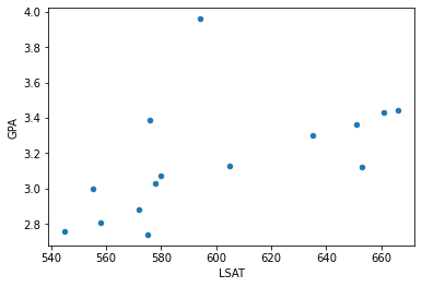
png
# Plug-in estimates for mean and correlation

X = df['LSAT'].to_numpy()
Y = df['GPA'].to_numpy()

def corr(X, Y):
    mu_x = X.mean()
    mu_y = Y.mean()

    return sum((X - mu_x) * (Y - mu_y)) / math.sqrt(sum((X - mu_x)**2) * sum((Y - mu_y)**2))


theta_hat = corr(X, Y)

print('Estimated correlation coefficient: %.4f' % corr(X, Y))
Estimated correlation coefficient: 0.5459# Bootstrap for SE of correlation coefficient
nx = len(X)
ny = len(Y)
B = 1000000
t_boot = np.empty(B)
for i in notebook.tqdm(range(B)):
xx = np.random.choice(X, nx, replace=True)
yy = np.random.choice(Y, ny, replace=True)
t_boot[i] = corr(xx, yy)
se = t_boot.std()
print('Estimated SE of correlation coefficient: %.4f' % se) 0%| | 0/1000000 [00:00<?, ?it/s]
Estimated SE of correlation coefficient: 0.2676# Confidence intervals obtained from bootstrap
from scipy.stats import norm
z = norm.ppf(.975)
normal_conf = (theta_hat - z * se, theta_hat + z * se)
percentile_conf = (np.quantile(t_boot, .025), np.quantile(t_boot, .975))
pivotal_conf = (2*theta_hat - np.quantile(t_boot, 0.975), 2*theta_hat - np.quantile(t_boot, .025))
print('95%% confidence interval (Normal): \t %.3f, %.3f' % normal_conf)
print('95%% confidence interval (percentile): \t %.3f, %.3f' % percentile_conf)
print('95%% confidence interval (pivotal): \t %.3f, %.3f' % pivotal_conf)95% confidence interval (Normal): 0.022, 1.070
95% confidence interval (percentile): -0.502, 0.523
95% confidence interval (pivotal): 0.569, 1.594Exercise 9.6.2. (Computer Experiment). Conduct a simulation to compare the four bootstrap confidence interval methods.
Let \(n = 50\) and let \(T(F) = \int (x - \mu)^3 dF(x) / \sigma^3\) be the skewness. Draw \(Y_1, \dots, Y_n \sim N(0, 1)\) and set \(X_i = e^{Y_i}\), \(i = 1, \dots, n\). Construct the four types of bootstrap 95% intervals for \(T(F)\) from the data \(X_1, \dots, X_n\). Repeat this whole thing many times and estimate the true coverage of the four intervals.
import numpy as np
from tqdm import notebook
from scipy.stats import norm

def create_data(n=50):
    y = norm.rvs(size=n)
    return np.exp(y)

def skewness(x):
    n = len(x)
    mu = sum(x) / n
    var = sum((x - mu)**2) / n
    return sum((x - mu)**3 / (n * var**(3/2)))

def bootstrap_values(x, B=10000, show_progress=True):
    n = len(x)
    t_boot = np.empty(B)
    iterable = notebook.tqdm(range(B)) if show_progress else range(B)
    for i in iterable:
        xx = np.random.choice(x, n, replace=True)
        t_boot[i] = skewness(xx)

    return t_boot

def bootstrap_intervals(theta_hat, t_boot, alpha=0.05):
    se = t_boot.std()

    z = norm.ppf(1 - alpha/2)
    q_half_alpha = np.quantile(t_boot, alpha/2)
    q_c_half_alpha = np.quantile(t_boot, 1 - alpha/2)

    normal_conf = (theta_hat - z * se, theta_hat + z * se)
    percentile_conf = (q_half_alpha, q_c_half_alpha)
    pivotal_conf = (2*theta_hat - q_c_half_alpha, 2*theta_hat - q_half_alpha)

    return normal_conf, percentile_conf, pivotal_conf
# Creating the data
x = create_data(n=50)# Nonparametric Bootstrap
theta_hat = skewness(x)
t_boot = bootstrap_values(x, B=100000)
normal_conf, percentile_conf, pivotal_conf = bootstrap_intervals(theta_hat, t_boot, alpha=0.05)
print('95%% confidence interval (Normal): \t %.3f, %.3f' % normal_conf)
print('95%% confidence interval (percentile): \t %.3f, %.3f' % percentile_conf)
print('95%% confidence interval (pivotal): \t %.3f, %.3f' % pivotal_conf) 0%| | 0/100000 [00:00<?, ?it/s]
95% confidence interval (Normal): 1.828, 7.650
95% confidence interval (percentile): 0.932, 5.490
95% confidence interval (pivotal): 3.988, 8.546Note: parametric bootstrap is only covered in chapter 10. The below assumes that “four types of bootstrap” in the exercise refers to the 3 types of nonparametric bootstrap covered in chapter 9, plus parametric bootstrap from chapter 10.
For the parametric bootstrap, assume \(X = e^Y\) where \(Y \sim N(\mu, \sigma^2)\).
The moment-generating function for a normal random variable Y is:
\[\begin{align}
M_X(t)=E(e^{tY})&=\frac{1}{\sqrt{2\pi}\sigma}\int_{-\infty}^{+\infty}e^{ty} e^{-\frac{1}{2}(\frac{y-\mu}{\sigma})^2}dy\\
&=\frac{1}{\sqrt{2\pi}\sigma}\int_{-\infty}^{+\infty}exp(-\frac{y^2-2y\mu+\mu^2-2\sigma^2ty}{2\sigma^2})dy\\
&=\frac{1}{\sqrt{2\pi}\sigma}\int_{-\infty}^{+\infty}exp(-\frac{(y-(\mu+t\sigma^2))^2-2t\mu\sigma^2-t^2\sigma^4}{2\sigma^2})dy\\
&=\frac{1}{\sqrt{2\pi}\sigma}exp(t\mu+t^2\sigma^2/2)\int_{-\infty}^{+\infty}exp(-\frac{1}{2}\frac{(y-(\mu+t\sigma^2))^2}{\sigma^2})dy\\
&=exp(t\mu+t^2\sigma^2/2)\frac{1}{\sqrt{2\pi}\sigma}\int_{-\infty}^{+\infty}exp\Biggl[-\frac{1}{2}\Bigl[\frac{y-(\mu+t\sigma^2)}{\sigma}\Bigr]^2\Biggr]dy\\
&=e^{t\mu+t^2\sigma^2/2}
\end{align}\]
Then
\[\begin{align} \mathbb{E}(X) &= \mathbb{E}(e^Y) \\ &= \int_{-\infty}^\infty e^y \frac{1}{\sigma \sqrt{2 \pi}} e^{-\frac{1}{2} \left(\frac{y - \mu}{\sigma} \right)^2} dy \\ &= \frac{1}{\sigma \sqrt{2 \pi}} \int e^{y - \frac{1}{2}\left(\frac{y - \mu}{\sigma}\right)^2} dy \\ &=\frac{1}{\sqrt{2\pi}\sigma}\int_{-\infty}^{+\infty}exp\left(-\frac{y^2-2y\mu+\mu^2-2\sigma^2y}{2\sigma^2}\right)dy \\ &=\frac{1}{\sqrt{2\pi}\sigma}\int_{-\infty}^{+\infty}exp\left(-\frac{(y-(\mu+\sigma^2))^2-2\mu\sigma^2-\sigma^4}{2\sigma^2}\right)dy \\ &=\frac{1}{\sqrt{2\pi}\sigma}exp(\mu+\sigma^2/2)\int_{-\infty}^{+\infty}exp\left(-\frac{1}{2}\frac{(y-(\mu+\sigma^2))^2}{\sigma^2}\right)dy \\ &=exp(\mu+\sigma^2/2)\frac{1}{\sqrt{2\pi}\sigma}\int_{-\infty}^{+\infty}exp\Biggl[-\frac{1}{2}\Bigl[\frac{y-(\mu+\sigma^2)}{\sigma}\Bigr]^2\Biggr]dy \\ &= e^{\mu + \sigma^2/2} \\ \end{align}\]
\[\mathbb{E}(X^2) = \mathbb{E}(e^{2Y}) = e^{2\mu + (2\sigma)^2/2} = e^{2\mu + 2\sigma^2}\]
Solving the two equations for the moments we get parameter estimates:
\[ \begin{align} \hat{\mu}_Y & = \left[4 \log \mathbb{E}(X) - \log \mathbb{E}(X^2)\right]/2 \\ \hat{\sigma}_Y & = \sqrt{\log \mathbb{E}(X^2) - 2 \log \mathbb{E}(X)} \end{align} \]
From these parameter estimates, we can generate bootstrap samples: sample values for \(Y_i ~ N(\hat{\mu}_Y, \hat{\sigma}_Y^2)\), calculate \(X_i = Y_i\), and calculate the statistic \(T(X_i)\) on each sample generated this way.
# Parametric bootstrap
# Assume X = e^Y, Y ~ N(\mu, \sigma^2)

def estimate_parameters(x):
    log_e_x = np.log(x.mean())
    log_e_x2 = np.log((x**2).mean())

    mu_Y_hat = (4 * log_e_x - log_e_x2)/2
    sigma_Y_hat = np.sqrt(log_e_x2 - 2 * log_e_x)

    return mu_Y_hat, sigma_Y_hat

def bootstrap_skewness_parametric(mu, sigma, n, B = 10000, show_progress=True):
    t_boot = np.empty(B)
    iterable = notebook.tqdm(range(B)) if show_progress else range(B)
    for i in iterable:
        xx = np.exp(norm.rvs(size=n, loc=n, scale=sigma))
        t_boot[i] = skewness(xx)

    return t_boot

def bootstrap_parametric_intervals(mu, t_boot, alpha=0.05):
    se = t_boot.std()
    z = norm.ppf(1 - alpha/2)

    return (theta_hat - z * se, theta_hat + z * se)
mu_X_hat = x.mean()
mu_Y_hat, sigma_Y_hat = estimate_parameters(x)
t_boot = bootstrap_skewness_parametric(mu_Y_hat, sigma_Y_hat, 50, B=100000)
parametric_normal_conf = bootstrap_parametric_intervals(mu_X_hat, t_boot, alpha=0.05)
print('95%% confidence interval (Parametric Normal): \t %.3f, %.3f' % parametric_normal_conf) 0%| | 0/100000 [00:00<?, ?it/s]
95% confidence interval (Parametric Normal): 2.513, 6.965# Repeat nonparametric bootstrap many times
n_experiments = 10
normal_conf = np.empty((n_experiments, 2))
percentile_conf = np.empty((n_experiments, 2))
pivotal_conf = np.empty((n_experiments, 2))
for i in notebook.tqdm(range(n_experiments)):
theta_hat = skewness(x)
t_boot_experiment = bootstrap_values(x, B=100000, show_progress=False)
normal_conf[i], percentile_conf[i], pivotal_conf[i] = bootstrap_intervals(theta_hat, t_boot_experiment, alpha=0.05) 0%| | 0/10 [00:00<?, ?it/s]print('Normal confidence lower bound: \t\t mean %.3f, SE %.3f' %
(normal_conf[:, 0].mean(), normal_conf[:, 0].std()))
print('Normal confidence upper bound: \t\t mean %.3f, SE %.3f' %
(normal_conf[:, 1].mean(), normal_conf[:, 1].std()))
print('Percentile confidence lower bound: \t mean %.3f, SE %.3f' %
(percentile_conf[:, 0].mean(), percentile_conf[:, 0].std()))
print('Percentile confidence upper bound: \t mean %.3f, SE %.3f' %
(percentile_conf[:, 1].mean(), percentile_conf[:, 1].std()))
print('Pivotal confidence lower bound: \t mean %.3f, SE %.3f' %
(pivotal_conf[:, 0].mean(), pivotal_conf[:, 0].std()))
print('Pivotal confidence upper bound: \t mean %.3f, SE %.3f' %
(pivotal_conf[:, 1].mean(), pivotal_conf[:, 1].std()))Normal confidence lower bound: mean 1.821, SE 0.005
Normal confidence upper bound: mean 7.657, SE 0.005
Percentile confidence lower bound: mean 0.928, SE 0.004
Percentile confidence upper bound: mean 5.494, SE 0.004
Pivotal confidence lower bound: mean 3.984, SE 0.004
Pivotal confidence upper bound: mean 8.550, SE 0.004# Repeat parametric bootstrap many times
n_experiments = 10
parametric_normal_conf = np.empty((n_experiments, 2))
for i in notebook.tqdm(range(n_experiments)):
mu_X_hat = x.mean()
mu_Y_hat, sigma_Y_hat = estimate_parameters(x)
t_boot = bootstrap_skewness_parametric(mu_Y_hat, sigma_Y_hat, 50, B=100000, show_progress=False)
parametric_normal_conf[i] = bootstrap_parametric_intervals(mu_X_hat, t_boot, alpha=0.05) 0%| | 0/10 [00:00<?, ?it/s]print('Parametric Normal confidence lower bound: \t mean %.3f, SE %.3f' %
(parametric_normal_conf[:, 0].mean(), parametric_normal_conf[:, 0].std()))
print('Parametric Normal confidence upper bound: \t mean %.3f, SE %.3f' %
(parametric_normal_conf[:, 1].mean(), parametric_normal_conf[:, 1].std()))Parametric Normal confidence lower bound: mean 2.512, SE 0.006
Parametric Normal confidence upper bound: mean 6.966, SE 0.006Exercise 9.6.3. Let \(X_1, \dots, X_n \sim t_3\) where \(n = 25\). Let \(\theta = T(F) = (q_{.75} - q_{.25})/1.34\) where \(q_p\) denotes the \(p\)-th quantile. Do a simulation to compare the coverage and length of the following confidence intervals for \(\theta\):
- Normal interval with standard error from the bootstrap
- Bootstrap percentile interval
Remark: the jacknife does not give a consistent estimator of the variance of a quantile.
Solution. We will assume that \(t_3\) represents a t-distribution with shape parameter 3.
import numpy as np
from scipy.stats import t
from tqdm import notebook

n = 25
X = t.rvs(3, size=25)
def T(x):
return (np.quantile(x, 0.75) - np.quantile(x, 0.25)) / 1.34theta_hat = T(X)# Run bootstrap
B = 1000000
t_boot = np.empty(B)
for i in notebook.tqdm(range(B)):
xx = np.random.choice(X, n, replace=True)
t_boot[i] = T(xx)
se_boot = t_boot.std()
alpha = 0.05
z = norm.ppf(1 - alpha/2)
q_half_alpha = np.quantile(t_boot, alpha/2)
q_c_half_alpha = np.quantile(t_boot, 1 - alpha/2)
normal_conf = (theta_hat - z * se_boot, theta_hat + z * se_boot)
percentile_conf = (q_half_alpha, q_c_half_alpha)
print('95%% confidence interval (Normal): \t %.3f, %.3f' % normal_conf)
print('95%% confidence interval (percentile): \t %.3f, %.3f' % percentile_conf) 0%| | 0/1000000 [00:00<?, ?it/s]
95% confidence interval (Normal): -0.072, 1.511
95% confidence interval (percentile): 0.422, 1.767Exercise 9.6.4. Let \(X_1, \dots, X_n\) be distinct observations (no ties). Show that there are
\[ \binom{2n - 1}{n}\]
distinct bootstrap samples.
Hint: Imagine putting \(n\) balls into \(n\) buckets.
Solution.
Each bootstrap sample (random draws with replacement) will select \(a_i\) copies of \(X_i\), where \(0 \leq a_i \leq n\) and \(\sum_{i=1}^n a_i = n\), for integer \(a_i\). Each bootstrap sample is uniquely represented by this sequence of variables, and each sequence of variables uniquely determines a bootstrap sample – so the number of distinct bootstrap samples is equal to the number of solutions to this equation, that is, the number of partitions of \(n\) into \(n\) buckets.
Lets write \(a_i\) explicitly in base 1, representing it as \(a_i\) consecutive copies of the digit 1:
\[ \begin{align} 0_{10} & = \text{empty string}_1 \\ 1_{10} & = 1_1 \\ 2_{10} & = 11_1 \\ 3_{10} & = 111_1 \\ 4_{10} & = 1111_1 \\ \vdots \end{align} \]
So a solution for
\[a_1 + a_2 + \dots + a_n = n\]
is uniquely represented by a sequence of \(2n - 1\) symbols, being \(n\) digits \(1\) and \(n - 1\) plus signs. For example, if \(a_1 = 3\), \(a_2 = 0\), \(a_3 = 1\), then we write
\[ 111 + + 1 + \dots = n \]
The number of such solutions is then obtained by choosing \(n\) of the \(2n - 1\) symbols to be digit \(1\) – that is, \(\binom{2n - 1}{n}\).
Exercise 9.6.5. Let \(X_1, \dots, X_n\) be distinct observations (no ties). Let \(X_1^*, \dots, X_n^*\) denote a bootstrap sample and let \(\overline{X}_n^* = n^{-1}\sum_{i=1}^nX_i^*\). Find:
- \(\mathbb{E}(\overline{X}_n^* | X_1, \dots, X_n)\)
- \(\mathbb{V}(\overline{X}_n^* | X_1, \dots, X_n)\)
- \(\mathbb{E}(\overline{X}_n^*)\)
- \(\mathbb{V}(\overline{X}_n^*)\)
Solution.
(a) \[ \begin{align} \mathbb{E}(\overline{X}_n^* | X_1, \dots, X_n) &= \mathbb{E}\left(n^{-1}\sum_{i=1}^nX_i\right) = n^{-1}\sum_{i=1}^n \mathbb{E}(X_i) = \mathbb{E}(X) \end{align} \]
(b) \[ \begin{align} \mathbb{V}(\overline{X}_n^* | X_1, \dots, X_n) & = \mathbb{E}((\overline{X}_n^*)^2 | X_1, \dots, X_n) - \mathbb{E}(\overline{X}_n^* | X_1, \dots, X_n)^2 \\ &= \mathbb{E}\left(\left(n^{-1}\sum_{i=1}^nX_i\right)^2\right) - \mathbb{E}\left(n^{-1}\sum_{i=1}^nX_i\right)^2 \\ &= n^{-2} \mathbb{E}\left(\sum_{i=1}^nX_i^2 + \sum_{i=1}^n \sum_{j=1, j \neq i}^n X_i X_j\right) - \mathbb{E}(X)^2 \\ &= n^{-2} \sum_{i=1}^n \mathbb{E}(X_i^2) + n^{-2} \sum_{i=1}^n \sum_{j=1, j \neq i}^n \mathbb{E}(X_i X_j) - \mathbb{E}(X)^2 \\ &= n^{-1} (\mathbb{V}(X) + \mathbb{E}(X)^2) + n^{-2} \sum_{i=1}^n \sum_{j=1, j \neq i}^n \mathbb{E}(X_i) \mathbb{E}(X_j) - \mathbb{E}(X)^2 \\ &= n^{-1} (\mathbb{V}(X) + \mathbb{E}(X)^2) + n^{-1} (n - 1) \mathbb{E}(X)^2 - \mathbb{E}(X)^2 \\ &= \frac{1}{n}\mathbb{V}(X) \end{align} \]
(c) \[ \begin{align} \mathbb{E}(\overline{X}_n^*) &= \mathbb{E}\left(n^{-1} \sum_{i=1}^nX_i^*\right) = n^{-1} \sum_{i=1}^n \mathbb{E}(X_i^*) = \mathbb{E}(X) \end{align} \]
(d) \[ \begin{align} \mathbb{V}(\overline{X}_n^*) &= \mathbb{E}((\overline{X}_n^*)^2) - \mathbb{E}(\overline{X}_n^*)^2 \\ &= \mathbb{E}\left(\left(n^{-1} \sum_{i=1}^nX_i^*\right)^2\right) - \mathbb{E}(X)^2 \\ &= n^{-2} \sum_{i=1}^n\sum_{j=1}^n \mathbb{E}(X_i^* X_j^*) - \mathbb{E}(X)^2 \end{align} \]
Now, the same value \(X_k\) may have been sampled twice in \(\mathbb{E}(X_i^* X_j^*)\). This always happens when \(i = j\), and this happens with probability \(1 / n\) when \(i \neq j\). Thus,
\[ \begin{align} \mathbb{V}(\overline{X}_n^*) &= n^{-2} \left(\sum_{i=1}^n \mathbb{E}(X_i^2) + \sum_{i=1}^n \sum_{j=1, j \neq i}^n \left( \frac{1}{n} \mathbb{E}(X_i^2) + \left(1 - \frac{1}{n}\right)\mathbb{E}(X_i)\mathbb{E}(X_j)\right) \right) - \mathbb{E}(X)^2 \\ &= n^{-1} \mathbb{E}(X^2) + n^{-2} (n-1) \mathbb{E}(X^2) + n^{-2}(n-1)^2 E(X)^2 - \mathbb{E}(X)^2 \\ &= n^{-2} (2n - 1) \left( \mathbb{E}(X^2) - \mathbb{E}(X)^2 \right) \\ &= \frac{2n - 1}{n^2} \mathbb{V}(X) \end{align} \]
Exercise 9.6.6. (Computer Experiment). Let \(X_1, \dots, X_n \sim N(\mu, 1)\). Let \(\theta = e^\mu\)and let \(\hat{\theta} = e^{\overline{X}}\) be the mle. Create a dataset (using \(\mu = 5\)) consisting of \(n = 100\) observations.
(a) Use the bootstrap to get the \(\text{se}\) and 95% confidence interval for \(\theta\).
(b) Plot a histogram of the bootstrap replications for the parametric and non-parametric bootstraps. These are estimates of the distribution of \(\hat{\theta}\). Compare this to the true sampling distribution of \(\hat{\theta}\).
import numpy as np
import pandas as pd
from scipy.stats import norm
from tqdm import notebook
%matplotlib inline

X = norm.rvs(loc=5, scale=1, size=100)
# Get estimated value
theta_hat = np.exp(X.mean())
# Run nonparametric bootstrap
B = 1000000
t_boot_nonparam = np.empty(B)
n = len(X)
for i in notebook.tqdm(range(B)):
xx = np.random.choice(X, n, replace=True)
t_boot_nonparam[i] = np.exp(xx.mean())
se_boot = t_boot_nonparam.std()
alpha = 0.05
z = norm.ppf(1 - alpha/2)
normal_conf = (theta_hat - z * se_boot, theta_hat + z * se_boot)
print('95%% confidence interval (Normal): \t %.3f, %.3f' % normal_conf) 0%| | 0/1000000 [00:00<?, ?it/s]
95% confidence interval (Normal): 128.387, 194.808# Run parametric bootstrap
mu_hat = X.mean()
theta_hat = np.exp(mu_hat)
B = 1000000
t_boot_param = np.empty(B)
n = len(X)
for i in notebook.tqdm(range(B)):
xx = norm.rvs(size=n, loc=mu_hat, scale=1)
t_boot_param[i] = np.exp(xx.mean())
se_boot_param = t_boot_param.std()
alpha = 0.05
z = norm.ppf(1 - alpha/2)
normal_conf_param = (theta_hat - z * se_boot_param, theta_hat + z * se_boot_param)
print('95%% confidence interval (Parametric Normal): \t %.3f, %.3f' % normal_conf_param) 0%| | 0/1000000 [00:00<?, ?it/s]
95% confidence interval (Parametric Normal): 129.688, 193.507For the true sampling distribution,
\[ \overline{X} = \frac{1}{n} \sum_{i=1}^n X_i \sim \frac{1}{n} N(n \mu, n) = N(\mu, n^{-2})\]
so the distribution of \(\hat{\theta}\) is the distribution of \(e^\overline{X}\). Its CDF is:
\[ \mathbb{P}\left(\hat{\theta} \leq t\right) = \mathbb{P}\left(e^\overline{X} \leq t\right) = \mathbb{P}\left(\overline{X} \leq \log t\right) = F_{\overline{X}}\left(\log t\right) \]
import numpy as np
from scipy.stats import norm
from matplotlib import pyplot

bins = np.linspace(50, 250, 500)
# Generate the CDF for theta, calculate it for each bin, and include the differences between bins
def theta_cdf(x):
return norm.cdf(np.log(x), loc=5, scale=1/50)
theta_cdf_bins = list(map(theta_cdf, bins))
theta_cdf_bins_delta = np.empty(len(bins))
theta_cdf_bins_delta[0] = 0
theta_cdf_bins_delta[1:] = np.diff(theta_cdf_bins)pyplot.figure(figsize=(12, 8))
pyplot.hist(t_boot_nonparam, bins, label='Nonparametric bootstrap', color='blue', histtype='step', density=True)
pyplot.hist(t_boot_param, bins, label='Parametric bootstrap', color='red', histtype='step', density=True)
pyplot.step(bins, theta_cdf_bins_delta, color='green', label='True sampling distribution')
pyplot.axvline(x=np.exp(5), color='black', label='θ (true parameter)')
pyplot.legend(loc='upper left')
pyplot.show()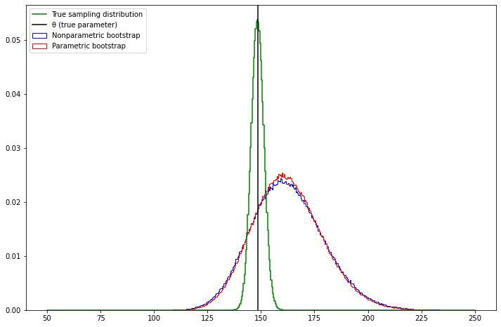
png
Exercise 9.6.7. Let \(X_1, \dots, X_n \sim \text{Uniform}(0, \theta)\). The mle is \(\hat{\theta} = X_\text{max} = \max \{ X_1, \dots, X_n \}\). Generate a dataset of size 50 with \(\theta = 1\).
(a) Find the distribution of \(\hat{\theta}\). Compare the true distribution of \(\hat{\theta}\) to the histograms from the parametric and nonparametric bootstraps.
(b) This is a case where the nonparametric bootstrap does very poorly. In fact, we can prove that this is the case. Show that, for parametric bootstrap \(\mathbb{P}(\hat{\theta}^* = \hat{\theta}) = 0\) but for the nonparametric \(\mathbb{P}(\hat{\theta}^* = \hat{\theta}) \approx 0.632\).
Hint: show that \(\mathbb{P}(\hat{\theta}^* = \hat{\theta}) = 1 - (1 - (1/n))^n\) then take the limit as \(n\) gets large.
import numpy as np

X = np.random.uniform(low=0, high=1, size=50)
# Nonparametric bootstrap
theta_hat = X.max()
B = 1000000
t_boot_nonparam = np.empty(B)
n = len(X)
for i in notebook.tqdm(range(B)):
xx = np.random.choice(X, n, replace=True)
t_boot_nonparam[i] = xx.max()
se_boot = t_boot_nonparam.std()
alpha = 0.05
z = norm.ppf(1 - alpha/2)
normal_conf = (theta_hat - z * se_boot, theta_hat + z * se_boot)
print('95%% confidence interval (Normal): \t %.3f, %.3f' % normal_conf) 0%| | 0/1000000 [00:00<?, ?it/s]
95% confidence interval (Normal): 0.979, 1.019# Run parametric bootstrap
theta_hat = X.max()
B = 1000000
t_boot_param = np.empty(B)
n = len(X)
for i in notebook.tqdm(range(B)):
xx = np.random.uniform(low=0, high=theta_hat, size=50)
t_boot_param[i] = xx.max()
se_boot_param = t_boot_param.std()
alpha = 0.05
z = norm.ppf(1 - alpha/2)
normal_conf_param = (theta_hat - z * se_boot_param, theta_hat + z * se_boot_param)
print('95%% confidence interval (Parametric Normal): \t %.3f, %.3f' % normal_conf_param) 0%| | 0/1000000 [00:00<?, ?it/s]
95% confidence interval (Parametric Normal): 0.961, 1.037For the true sampling distribution,
\[\hat{\theta} = \max \{ X_1, \dots X_n \}\]
Its CDF is
\[\mathbb{P}(\hat{\theta} \leq x) = \prod_{i=1}^n \mathbb{P}(X_i \leq x) = F_{\text{Uniform}(0, \theta)}(x)^n\]
where
\[F_{\text{Uniform}(0, \theta)}(x) = \begin{cases} 0 & \text{if } x \leq 0 \\ \frac{x}{\theta} & \text{if } 0 < x \leq \theta \\ 1 & \text{if } \theta < x \end{cases} \]
bins = np.linspace(0.75, 1.05, 200)# Generate the CDF for theta, calculate it for each bin, and include the differences between bins
def theta_cdf(x):
if x <= 0:
return 0
if x >= 1:
return 1
return x**50
theta_cdf_bins = list(map(theta_cdf, bins))
theta_cdf_bins_delta = np.empty(len(bins))
theta_cdf_bins_delta[0] = 0
theta_cdf_bins_delta[1:] = np.diff(theta_cdf_bins)pyplot.figure(figsize=(12, 8))
pyplot.hist(t_boot_nonparam, bins, label='Nonparametric bootstrap', color='blue', histtype='step', density=True)
pyplot.hist(t_boot_param, bins, label='Parametric bootstrap', color='red', histtype='step', density=True)
pyplot.axvline(x=1, color='black', label='θ (true parameter)')
pyplot.legend(loc='upper left')
pyplot.show()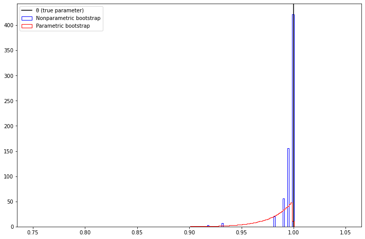
png
pyplot.figure(figsize=(12, 8))
pyplot.step(bins, theta_cdf_bins_delta, color='green', label='True sampling distribution')
pyplot.axvline(x=1, color='black', label='θ (true parameter)')
pyplot.legend(loc='upper left')
pyplot.ylim(0, 0.1)
pyplot.show()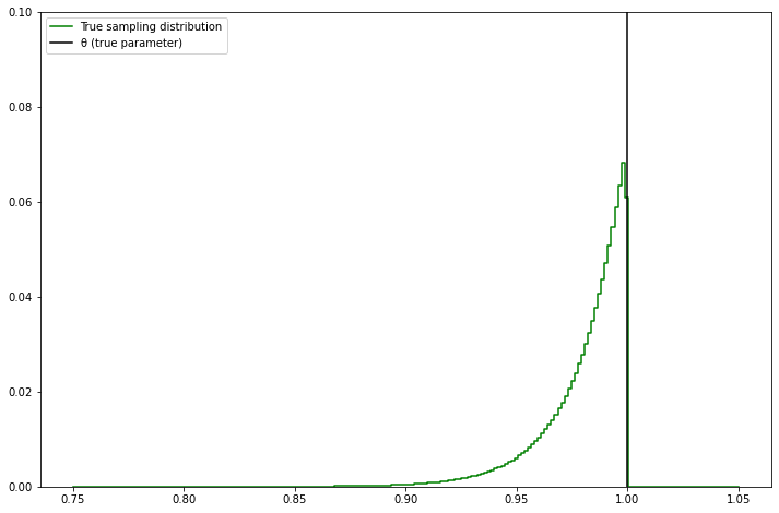
png
(b)
For the parametric bootstrap process, the estimated parameter \(\hat{\theta}^*\) is used on each \(k\)-th bootstrap sampling \(\{ X_{k1}, X_{k2}, \dots, X_{kn} \}\). But each variable \(X_{kj}\) is sampled from \(\text{Uniform}(0, \hat{\theta}^*)\), which is a continuous distribution – so the probability of obtaining exactly a sample at the boundaries is 0, and \(\mathbb{P}(X_{kj} < \hat{\theta}^*) = 1\). Since the bootstrap functional of each draw, \(T(F_n) = \max(F_n)\) is the largest drawn value in each sample, its values will also always be under \(\hat{\theta}\), thus the estimated parameter via parametric bootstraping will aywals be under \([\hat{\theta}\), and \(\mathbb{P}(\hat{\theta}* = \hat{\theta}) = 0\)].
For the nonparametric bootstrap process, the estimated parameter \(\hat{\theta}^*\) is the maximum value with a point mass in the empirical distribution function \(\hat{F}\). Each bootstrap resample may or may not include that value when drawing from this sample – if \(\max\{X_1, \dots, X_n\} \in \{X_{k1}, \dots, X_{kn} \}\) then the estimated functional for that bootstrap sample will be the estimated parameter \(\hat{\theta}^*\), otherwise it will necessarily be smaller.
Thus, the probability that \(\mathbb{P}(\hat{\theta}* = \hat{\theta})\) is the probability that the largest element on the original data is included in a resampling with replacement. That turns out to be one minus the probability that it never gets included, so, \(\mathbb{P}(\hat{\theta}* = \hat{\theta}) = 1 - (1 - (1/n))^n\). But \(\lim_{n \rightarrow \infty } (1 + x/n)^n = e^x\), so the given probability goes to \(1 - e^{-1} \approx 0.632\).
Exercise 9.6.8. Let \(T_n = \overline{X}_n^2\), \(\mu = \mathbb{E}(X_1)\), \(\alpha_k = \int |x - \mu|^k dF(x)\) and \(\hat{\alpha}_k = n^{-1} \sum_{i=1}^n |X_i - \overline{X}_n|^k\). Show that
\[v_\text{boot} = \frac{4 \overline{X}_n^2 \hat{\alpha}_2}{n} + \frac{4 \overline{X}_n \hat{\alpha}_3}{n^2} + \frac{\hat{\alpha}_4}{n^3}\]
Solution.
First, we rewrite the sample mean in terms of an expression containing the central moments. Let \(S_n = n^{-1} \sum_{i=1}^n (X_i - \overline{X}_n) = 0\). Then:
\[ \overline{X}_n = S_n + \overline{X}_n = \frac{1}{n} \sum_{i=1}^n (X_i - \overline{X}_n) + \overline{X}_n \]
The bootstrap variance, \(\mathbb{V}\left(\overline{X}_n^2\right)\), can be expressed as
\[ \mathbb{V}\left(\overline{X}_n^2\right) = \mathbb{E}\left(\overline{X}_n^4\right) - \mathbb{E}\left(\overline{X}_n^2\right)^2 \]
Note that \(\overline{X}_n\) is the mean of the distribution, and can be treated as constant when taking expectations.
We now have:
\[ \begin{align} \mathbb{E}\left(\overline{X}_n^4\right) &= \mathbb{E}\left( (S_n + \overline{X}_n)^4 \right) \\ &= \mathbb{E}\left( S_n^4 + 4 S_n^3 \overline{X}_n + 6 S_n^2 \overline{X}_n^2 + 4 S_n \overline{X}_n^3 + \overline{X}_n^4 \right) \\ &= \mathbb{E}(S_n^4) + 4 \overline{X}_n \mathbb{E}(S_n^3) + 6 \overline{X}_n^2 \mathbb{E}(S_n^2) + 4 \overline{X}_n^3 \mathbb{E}(S_n) + \overline{X}_n^4 \end{align} \]
Then, computing the moments of \(S_n\),
\[ \begin{align} \mathbb{E}(S_n) &= 0 \\ \mathbb{E}(S_n^2) &= \mathbb{E}\left( n^{-2} \left( \sum_i X_i - \overline{X}_n \right)^2 \right) = \frac{\hat{\alpha}_2}{n} \\ \mathbb{E}(S_n^3) &= \mathbb{E}\left( n^{-3} \left( \sum_i X_i - \overline{X}_n \right)^3 \right) = \frac{\hat{\alpha}_3}{n^2} \\ \mathbb{E}(S_n^4) &= \mathbb{E}\left( n^{-4} \left( \sum_i X_i - \overline{X}_n \right)^4 + n^{-2}n^{-4} \sum_i \sum_{j \neq i} (X_i - \overline{X}_n)^2 (X_j - \overline{X}_n)^2 \right) = \frac{\hat{\alpha}_4 + \hat{\alpha}_2^2}{n^3} \end{align} \]
and finally
\[ \mathbb{E}\left(\overline{X}_n^2\right)^2 = \mathbb{E}\left(\overline{X}_n^2 + S_n\right)^2 = \overline{X}_n^4 + 2 \overline{X}_n^2 \frac{\hat{\alpha}_2}{n} + \frac{\hat{\alpha}_2^2}{n^2} \]
Putting everything together,
\[ \begin{align} v_\text{boot} &= \mathbb{E}\left( (S_n + \overline{X}_n)^4 \right) - \mathbb{E}\left(\overline{X}_n^2 + S_n\right)^2 \\ &= \mathbb{E}(S_n^4) + 4 \overline{X}_n \mathbb{E}(S_n^3) + 6 \overline{X}_n^2 \mathbb{E}(S_n^2) + 4 \overline{X}_n^3 \mathbb{E}(S_n) + \overline{X}_n^4 - \left( \overline{X}_n^4 + 2 \overline{X}_n^2 \frac{\hat{\alpha}_2}{n} + \frac{\hat{\alpha}_2^2}{n^2}\right) \\ &= \frac{\hat{\alpha}_4 + \hat{\alpha}_2^2}{n^3} + 4 \overline{X}_n \frac{\hat{\alpha}_3}{n^2} + 6 \overline{X}_n^2 \frac{\hat{\alpha}_2}{n} + 0 + \overline{X}_n^4 - \overline{X}_n^4 - 2 \overline{X}_n^2 \frac{\hat{\alpha}_2}{n} - \frac{\hat{\alpha}_2^2}{n^2} \\ &= \frac{4 \overline{X}_n^2 \hat{\alpha}_2}{n} + \frac{4 \overline{X}_n \hat{\alpha}_3}{n^2} + \frac{\hat{\alpha}_4}{n^3} \end{align} \]
Reference and discussion: https://stats.stackexchange.com/q/26082