8. Estimating the CDF and Statistical Functionals
8.1 Empirical distribution function
The empirical distribution function \(\hat{F_n}\) is the CDF that puts mass \(1/n\) at each data point \(X_i\). Formally,
\[ \begin{align} \hat{F_n}(x) & = \frac{\sum_{i=1}^n I\left(X_i \leq x \right)}{n} \\ &= \frac{\text{#}|\text{observations less than or equal to x}|}{n} \end{align} \]
where
\[ \begin{equation} I\left(X_i \leq x\right) = \begin{cases} 1 & \text{if } X_i \leq x \\ 0 & \text{if } X_i > x \end{cases} \end{equation} \]
Theorem 8.3. At any fixed value of \(x\),
\[ \begin{equation} \mathbb{E}\left( \hat{F_n}(x) \right) = F(x) \quad\mathrm{and}\quad \mathbb{V}\left( \hat{F_n}(x) \right) = \frac{F(x)(1 - F(x))}{n} \end{equation} \]
Thus,
\[ \text{MSE} = \frac{F(x)(1 - F(x))}{n} \rightarrow 0 \]
and hence, \(\hat{F_n}(x) \xrightarrow{\text{P}} F(x)\).
Theorem 8.4 (Glivenko-Cantelli Theorem). Let \(X_1, \dots, X_n \sim F\). Then
\[ \sup _x |\hat{F_n}(x) - F(x)| \xrightarrow{\text{P}} 0 \]
(actually, \(\sup _x |\hat{F_n}(x) - F(x)|\) converges to 0 almost surely.)
8.2 Statistical Functionals
A statistical functional \(T(F)\) is any function of \(F\). Examples are the mean \(\mu = \int x dF(x)\), the variance \(\sigma^2 = \int (x - \mu)^2 dF(x)\) and the median \(m = F^{-1}(1/2)\).
The plug-in estimator of \(\theta = T(F)\) is defined by
\[\hat{\theta_n} = T(\hat{F_n}) \]
In other words, just plug in \(\hat{F_n}\) for the unknown \(F\).
A functional of the form \(\int r(x) dF(x)\) is called a linear functional. Recall that \(\int r(x) dF(x)\) is defined to be \(\int r(x) f(x) d(x)\) in the continuous case and \(\sum_j r(x_j) f(x_j)\) in the discrete.
The plug-in estimator for the linear functional \(T(F) = \int r(x) dF(x)\) is:
\[T(\hat{F_n}) = \int r(x) d\hat{F_n}(x) = \frac{1}{n} \sum_{i=1}^n r(X_i)\]
We have:
\[ T(\hat{F_n}) \approx N\left(T(F), \hat{\text{se}}\right) \]
An approximate \(1 - \alpha\) confidence interval for \(T(F)\) is then
\[ T(\hat{F_n}) \pm z_{\alpha/2} \hat{\text{se}} \]
We call this the Normal-based interval.
8.3 Technical Appendix
Theorem 8.12 (Dvoretsky-Kiefer-Wolfowitz (DKW) inequality). Let \(X_1, \dots, X_n\) be iid from \(F\). Then, for any \(\epsilon > 0\),
\[\mathbb{P}\left( \sup_x |F(x) - \hat{F_n}(x) | > \epsilon \right) \leq 2 e^{-2n\epsilon^2}\]
From the DKW inequality, we can construct a confidence set. Let \(\epsilon_n^2 = \log(2/\alpha) / (2n)\), \(L(x) = \max \{ \hat{F_n}(x) - \epsilon_n, \; 0 \}\) and \(U(x) = \min \{\hat{F_n}(x) + \epsilon_n, 1 \}\). It follows that for any \(F\),
\[ \mathbb{P}(F \in C_n) \geq 1 - \alpha \]
To summarize:
A \(1 - \alpha\) nonparametric confidence band for \(F\) is \((L(x), \; U(x))\) where
\[ \begin{align} L(x) &= \max \{ \hat{F_n}(x) - \epsilon_n, \; 0 \} \\ U(x) &= \min \{ \hat{F_n}(x) + \epsilon_n, \; 1 \} \\ \epsilon_n &= \sqrt{\frac{1}{2n} \log \left( \frac{2}{\alpha} \right) } \end{align} \]
8.5 Exercises
Exercise 8.5.1. Prove Theorem 8.3.
Solution. We have:
\[ \hat{F_n}(x) = \frac{\sum_{i=1}^n I\left(X_i \leq x \right)}{n} \]
where
\[ \begin{equation} I\left(X_i \leq x\right) = \begin{cases} 1 & \text{if } X_i \leq x \\ 0 & \text{if } X_i > x \end{cases} \end{equation} \]
Thus,
\[ \begin{align} \mathbb{E}(\hat{F_n}(x)) & = n^{-1} \sum_{i = 1}^n \mathbb{E}(I\left(X_i \leq x \right)) \\ & = n^{-1} \sum_{i = 1}^n \mathbb{P}\left(X_i \leq x \right) \\ & = n^{-1} \sum_{i = 1}^n F(x) \\ & = F(x) \end{align} \]
\[ \begin{align} \mathbb{E}(\hat{F_n}(x)^2) & = n^{-2} \mathbb{E} \left( \sum_{i = 1}^n I\left(X_i \leq x \right) \right)^2 \\ & = n^{-2} \mathbb{E} \left( \sum_{i = 1}^n I\left(X_i \leq x \right)^2 + \sum_{i = 1}^n \sum_{j = 1, j \neq i}^n I\left(X_i \leq x \right) I\left(X_j \leq x \right) \right) \\ & = n^{-2} \left( \sum_{i = 1}^n \mathbb{E} \left( I\left(X_i \leq x \right)^2 \right) + \sum_{i = 1}^n \sum_{j = 1, j \neq i}^n \mathbb{E} \left( I\left(X_i \leq x \right) I\left(X_j \leq x \right) \right) \right) \\ & = n^{-2} \left( \sum_{i = 1}^n \mathbb{E} \left( I\left(X_i \leq x \right) \right) + \sum_{i = 1}^n \sum_{j = 1, j \neq i}^n \mathbb{E} \left( I\left(X_i \leq x \right) \right) \mathbb{E} \left( I\left(X_j \leq x \right) \right) \right) \\ & = n^{-2} \left( \sum_{i = 1}^n \mathbb{P}\left(X_i \leq x \right) + \sum_{i = 1}^n \sum_{j = 1, j \neq i}^n \mathbb{P}\left(X_i \leq x \right) \mathbb{P}\left(X_j \leq x \right) \right) \\ &= n^{-2} \left( \sum_{i = 1}^n F(x) + \sum_{i = 1}^n \sum_{j = 1, j \neq i}^n F(x)^2 \right) \\ &= n^{-2} \left( nF(x) + (n^2 - n)F(x)^2 \right) \\ &= n^{-1} ( F(x) + (n - 1) F(x)^2 ) \end{align} \]
Therefore,
\[ \mathbb{V}(\hat{F_n}(x)) = \mathbb{E}(\hat{F_n}(x)^2) - \mathbb{E}(\hat{F_n}(x))^2 = F(x) /n + (1 - 1/n)F(x)^2 - F(x)^2 = \frac{F(x)(1 - F(x))}{n} \]
Finally,
\[ \text{MSE} = (\text{bias}(\hat{F_n}(x)))^2 + \mathbb{V}(\hat{F_n}(x)) \\ = (\mathbb{E}(\hat{F_n}(x)) - F(x))^2 + \mathbb{V}(\hat{F_n}(x)) = \mathbb{V}(\hat{F_n}(x)) = \frac{F(x)(1 - F(x))}{n} \rightarrow 0\]
Exercise 8.5.2. Let \(X_1, \dots, X_n \sim \text{Bernoulli}(p)\) and let \(Y_1, \dots, Y_m \sim \text{Bernoulli}(q)\).
- Find the plug-in estimator and estimated standard error for \(p\).
- Find an approximate 90-percent confidence interval for \(p\).
- Find the plug-in estimator and estimated standard error for \(p - q\).
- Find an approximate 90-percent confidence interval for \(p - q\).
Solution.
(a)
\(p\) is the mean of \(\text{Bernoulli}(p)\), so its plugin estimator is \(\hat{p} = \mathbb{E}(\hat{F_n}) = n^{-1} \sum_{i=1}^n X_i = \overline{X}_n\).
\(\sqrt{p(1-p)}\) is the standard error of \(\text{Bernoulli}(p)\), so its plugin estimator is \(\sqrt{\hat{p}(1-\hat{p})} = \sqrt{\overline{X}_n(1 - \overline{X}_n)}\).
(b)
The 90-percent confidence interval for \(p\) is \(\hat{p} \pm z_{5\%} \hat{se}(\hat{p})= \overline{X}_n \pm z_{5\%} \sqrt{\overline{X}_n(1-\overline{X}_n)}\).
(c)
The plug-in estimator for \(\theta = p - q\) is \(\hat{\theta} = \hat{p} - \hat{q} = \overline{X}_n - \overline{Y}_m\).
The standard error of \(\hat{\theta}\) is
\[\text{se} = \sqrt{\mathbb{V}(\hat{p} - \hat{q})} = \sqrt{\mathbb{V}(\hat{p}) + \mathbb{V}(\hat{q})} = \sqrt{\hat{p}(1 - \hat{p}) + \hat{q}(1 - \hat{q})} = \sqrt{\overline{X}_n(1 - \overline{X}_n) + \overline{Y}_m(1 - \overline{Y}_m)} \]
(d)
The 90-percent confidence interval for \(\theta = p - q\) is $ z_{5%} () = _n - m z{5%} $
Exercise 8.5.3. (Computer Experiment) Generate 100 observations from a \(N(0, 1)\) distribution. Compute a 95 percent confidence band for the CDF \(F\). Repeat this 1000 times and see how often the confidence band contains the true function. Repeat using data from a Cauchy distribution.
import math
import numpy as np
import pandas as pd
from scipy.stats import norm, cauchy
import matplotlib.pyplot as plt
from tqdm import notebook
# One iteration wtih Normal distribution
n = 100
alpha = 0.05
r = norm.rvs(size=n)
epsilon = math.sqrt((1 / (2 * n)) * math.log(2 / alpha))
F_n = lambda x : sum(r < x) / n
L_n = lambda x : max(F_n(x) - epsilon, 0)
U_n = lambda x : min(F_n(x) + epsilon, 1)
xx = sorted(r)
df = pd.DataFrame({
'x': xx,
'F_n': np.array(list(map(F_n, xx))),
'U_n': np.array(list(map(U_n, xx))),
'L_n': np.array(list(map(L_n, xx))),
'CDF': np.array(list(map(norm.cdf, xx)))
})
df['in_bounds'] = (df['U_n'] >= df['CDF']) & (df['CDF'] >= df['L_n'])
plt.plot( 'x', 'L_n', data=df, color='red')
plt.plot( 'x', 'U_n', data=df, color='green')
plt.plot( 'x', 'CDF', data=df, color='purple')
plt.legend()<matplotlib.legend.Legend at 0x7f2580e620a0>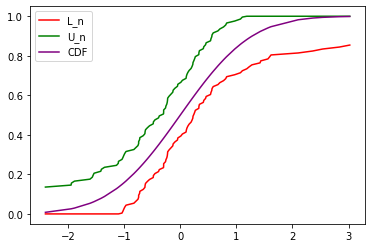
png
# 1000 iterations with Normal distribution

bounds = []
for k in notebook.tqdm(range(1000)):
    n = 100
    alpha = 0.05
    r = norm.rvs(size=n)
    epsilon = math.sqrt((1 / (2 * n)) * math.log(2 / alpha))

    F_n = lambda x : sum(r < x) / n
    L_n = lambda x : max(F_n(x) - epsilon, 0)
    U_n = lambda x : min(F_n(x) + epsilon, 1)

    # xx = sorted(r)
    xx = r # No need to sort without plotting

    df = pd.DataFrame({
        'x': xx,
        'F_n': np.array(list(map(F_n, xx))),
        'U_n': np.array(list(map(U_n, xx))),
        'L_n': np.array(list(map(L_n, xx))),
        'CDF': np.array(list(map(norm.cdf, xx)))
    })
    all_in_bounds = ((df['U_n'] >= df['CDF']) & (df['CDF'] >= df['L_n'])).all()
    bounds.append(all_in_bounds)

print('Average fraction in bounds: %.3f' % np.array(bounds).mean())
0%| | 0/1000 [00:00<?, ?it/s]
Average fraction in bounds: 0.965# One iteration wtih Cauchy distribution
n = 100
alpha = 0.05
r = cauchy.rvs(size=n)
epsilon = math.sqrt((1 / (2 * n)) * math.log(2 / alpha))
F_n = lambda x : sum(r < x) / n
L_n = lambda x : max(F_n(x) - epsilon, 0)
U_n = lambda x : min(F_n(x) + epsilon, 1)
xx = sorted(r)
df = pd.DataFrame({
'x': xx,
'F_n': np.array(list(map(F_n, xx))),
'U_n': np.array(list(map(U_n, xx))),
'L_n': np.array(list(map(L_n, xx))),
'CDF': np.array(list(map(norm.cdf, xx)))
})
df['in_bounds'] = (df['U_n'] >= df['CDF']) & (df['CDF'] >= df['L_n'])
plt.plot( 'x', 'L_n', data=df, color='red')
plt.plot( 'x', 'U_n', data=df, color='green')
plt.plot( 'x', 'CDF', data=df, color='purple')
plt.legend()<matplotlib.legend.Legend at 0x7f0394ce8dc0>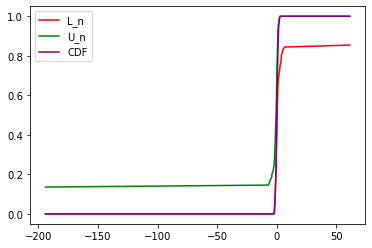
png
# 1000 iterations with Cauchy distribution

bounds = []
for k in tqdm.notebook.tqdm(range(1000)):
    n = 100
    alpha = 0.05
    r = cauchy.rvs(size=n)
    epsilon = math.sqrt((1 / (2 * n)) * math.log(2 / alpha))

    F_n = lambda x : sum(r < x) / n
    L_n = lambda x : max(F_n(x) - epsilon, 0)
    U_n = lambda x : min(F_n(x) + epsilon, 1)

    # xx = sorted(r)
    xx = r # No need to sort without plotting

    df = pd.DataFrame({
        'x': xx,
        'F_n': np.array(list(map(F_n, xx))),
        'U_n': np.array(list(map(U_n, xx))),
        'L_n': np.array(list(map(L_n, xx))),
        'CDF': np.array(list(map(norm.cdf, xx)))
    })
    all_in_bounds = ((df['U_n'] >= df['CDF']) & (df['CDF'] >= df['L_n'])).all()
    bounds.append(all_in_bounds)

print('Average fraction in bounds: %.3f' % np.array(bounds).mean())
0%| | 0/1000 [00:00<?, ?it/s]
Average fraction in bounds: 0.192Exercise 8.5.4. Let \(X_1, \dots, X_n \sim F\) and let \(\hat{F}_n(x)\) be the empirical distribution function. For a fixed \(x\), use the central limit theorem to find the limiting distribution of \(\hat{F}_n(x)\).
Solution.
We have:
\[ \hat{F_n}(x) = \frac{\sum_{i=1}^n I\left(X_i \leq x \right)}{n} \]
where
\[ \begin{equation} I\left(X_i \leq x\right) = \begin{cases} 1 & \text{if } X_i \leq x \\ 0 & \text{if } X_i > x \end{cases} \end{equation} \]
Let \(Y_i = I\left(X_i \leq x \right)\) for some fixed \(x\). From the central limit theorem,
\[ \begin{align} \sqrt{n} (\overline{Y}_n - \mu_Y) & \leadsto N(0, \sigma_Y^2) \\ \overline{Y}_n & \leadsto N(\mu_Y, \sigma_Y^2 / n) \end{align} \]
We can estimate the mean \(\mu_Y\) as \(\mathbb{E}(\hat{\mu_Y}) = \mathbb{E}(\overline{Y}_n) = n^{-1} \sum_{i=1}^n \mathbb{E}(I(X_i \leq x)) = n^{-1} \sum_{i=1}^n F(x) = \hat{F_n}(x)\).
We can estimate the variance \(\sigma_Y^2\) as \[\mathbb{E}(\hat{\sigma_Y}^2) = \mathbb{E}(\mathbb{V}(\overline{Y}_n)) = n^{-1} \sum_{i=1}^n \mathbb{E}((Y_i - \overline{Y}_n)^2) \\ = n^{-1} \sum_{i=1}^n \left( \mathbb{E}(Y_i^2) - 2 \mathbb{E}(Y_i \overline{Y}_n) + \mathbb{E}(\overline{Y}_n^2) \right) \leq n^{-1} \sum_{i=1}^n \left( \mathbb{E}(Y_i) + \mathbb{E}(\overline{Y}_n^2) \right) \leq 2\]
Therefore, for large \(n\), the limiting distribution has variance that goes to 0 – so \(\overline{Y}_n \leadsto \mu_Y\), or \(I\left(X_i \leq x \right) \leadsto F(x)\) for every x. Then,
\(\hat{F_n}(x) \leadsto n^{-1} \sum_{i=1}^n F(x) = F(x)\),
and, as expected, \(F\) is the limiting distribution of \(F_n\).
Exercise 8.5.5. Let \(x\) and \(y\) be two distinct points. Find \(\text{Cov}(\hat{F_n}(x), \hat{F_n}(y))\).
Solution.
We have:
\[ \begin{align} \text{Cov}(\hat{F_n}(x), \hat{F_n}(y)) & = \mathbb{E}(\hat{F_n}(x) \hat{F_n}(y)) - \mathbb{E}(\hat{F_n}(x))\mathbb{E}(\hat{F_n}(y)) \\ &= \mathbb{E}(\hat{F_n}(x) \hat{F_n}(y)) - F(x)F(y) \end{align} \]
But:
\[ \hat{F_n}(x) \hat{F_n}(y) = \frac{1}{n^2} \sum_{i=1}^n \sum_{j=1}^n I(X_i \leq x) I(X_j \leq y) \]
so
\[ \begin{align} \mathbb{E}(\hat{F_n}(x) \hat{F_n}(y)) & = \frac{1}{n^2} \sum_{i=1}^n \sum_{j=1}^n \mathbb{E}(I(X_i \leq x) I(X_j \leq y)) \\ &= \frac{1}{n^2} \sum_{i=1}^n \sum_{j=1}^n \mathbb{P}(X_i \leq x, X_j \leq y) \\ &= \frac{1}{n^2} \sum_{i=1}^n \sum_{j=1}^n \mathbb{P}(X_i \leq x | X_j \leq y) \mathbb{P}(X_j \leq y) \\ &= \frac{1}{n^2} \left( \sum_{i=1}^n F(\min\{x, y\}) + \sum_{i=1}^n \sum_{j=1, j \neq i}^n F(x)F(y) \right) \\ &= \frac{1}{n} F(\min\{x, y\}) + \left( 1 - \frac{1}{n}\right) F(x)F(y) \end{align} \]
Therefore, assuming \(x \leq y\),
\[ \begin{align} \text{Cov}(\hat{F_n}(x), \hat{F_n}(y)) & = \mathbb{E}(\hat{F_n}(x) \hat{F_n}(y)) - \mathbb{E}(\hat{F_n}(x))\mathbb{E}(\hat{F_n}(y)) \\ &= \mathbb{E}(\hat{F_n}(x) \hat{F_n}(y)) - F(x)F(y) \\ &= \frac{1}{n} F(\min\{x, y\}) + \left( 1 - \frac{1}{n}\right) F(x)F(y) - F(x)F(y) \\ &= \frac{F(x)(1 - F(y))}{n} \end{align} \]
Exercise 8.5.6. Let \(X_1, \dots, X_n \sim F\) and let \(\hat{F}\) be the empirical distribution function. Let \(a < b\) be fixed numbers and define \(\theta = T(F) = F(b) - F(a)\). Let \(\hat{\theta} = T(\hat{F}_n) = \hat{F}_n(b) - \hat{F}_n(a)\).
- Find the estimated standard error of \(\hat{\theta}\).
- Find an expression for an approximate \(1 - \alpha\) confidence interval for \(\theta\).
Solution.
(a)
The estimated mean for \(\hat{\theta}\) is \(\mathbb{E}(\hat{\theta}) = \mathbb{E}(\hat{F}_n(b) - \hat{F}_n(a)) = \mathbb{E}(\hat{F}_n(b)) - \mathbb{E}(\hat{F}_n(a)) = F(b) - F(a) = \theta\).
The estimated variance for \(\hat{\theta}\) is
\[ \mathbb{V}(\hat{\theta}) = \mathbb{E}(\hat{\theta}^2) - \mathbb{E}(\hat{\theta})^2 \]
But
\[ \begin{align} \mathbb{E}(\hat{\theta}^2) & = \mathbb{E}((\hat{F}_n(b) - \hat{F}_n(a))^2) \\ &= \mathbb{E}(\hat{F}_n(a)^2 + \hat{F}_n(b)^2 - 2 \hat{F}_n(a)\hat{F}_n(b)) \\ &= \mathbb{E}(\hat{F}_n(a)^2) + \mathbb{E}(\hat{F}_n(b)^2) - 2 \mathbb{E}(\hat{F}_n(a)\hat{F}_n(b)) \end{align} \]
\[ \begin{align} \mathbb{E}(\hat{F}_n(a)^2) & = \mathbb{E}\left(\left(\frac{1}{n} \sum_{i=1}^n I(X_i \leq a)\right)^2\right) \\ & = \frac{1}{n^2} \left(\sum_{i=1}^n \mathbb{E} \left( I(X_i \leq a)^2 \right) + \sum_{i=1}^n \sum_{j=1, j \neq i}^n \mathbb{E}\left( I(X_i \leq a) I(X_j \leq a) \right) \right) \\ & = \frac{1}{n^2} \left(\sum_{i=1}^n \mathbb{E} \left( I(X_i \leq a) \right) + \sum_{i=1}^n \sum_{j=1, j \neq i}^n \mathbb{E}\left( I(X_i \leq a) I(X_j \leq a) \right) \right) \\ & = \frac{1}{n^2} \left(\sum_{i=1}^n \mathbb{P} \left( X_i \leq a \right) + \sum_{i=1}^n \sum_{j=1, j \neq i}^n \mathbb{P}\left( X_i \leq a, X_j \leq a \right) \right) \\ & = \frac{1}{n^2} \left(n F(a) + n(n-1) F(a)^2 \right) \\ &= F(a) \frac{1}{n} + F(a)^2 \left(1 - \frac{1}{n} \right) \\ \mathbb{E}(\hat{F}_n(b)^2) & = F(b) \frac{1}{n} + F(b)^2 \left(1 - \frac{1}{n} \right) \end{align} \]
From the previous exercise,
\[ \mathbb{E}(\hat{F}_n(a)\hat{F}_n(b)) = \frac{1}{n} F(a) + \left( 1 - \frac{1}{n}\right) F(a)F(b) \]
Putting it together,
\[ \begin{align} \mathbb{E}(\hat{\theta}^2) &= \mathbb{E}(\hat{F}_n(a)^2) + \mathbb{E}(\hat{F}_n(b)^2) - 2 \mathbb{E}(\hat{F}_n(a)\hat{F}_n(b)) \\ &= F(a) \frac{1}{n} + F(a)^2 \left(1 - \frac{1}{n} \right) + F(b) \frac{1}{n} + F(b)^2 \left(1 - \frac{1}{n} \right) - 2 \left( \frac{1}{n} F(a) + \left( 1 - \frac{1}{n}\right) F(a)F(b) \right) \\ &= \frac{1}{n} \left(F(b) - F(a)\right) + \left( 1 - \frac{1}{n}\right) \left( F(b) - F(a) \right)^2 \\ &= \frac{1}{n} \theta + \left( 1 - \frac{1}{n} \right) \theta^2 \\ \mathbb{V}(\hat{\theta}) &= \mathbb{E}(\hat{\theta}^2) - \mathbb{E}(\hat{\theta})^2 \\ &= \frac{1}{n} \theta + \left( 1 - \frac{1}{n} \right) \theta^2 - \theta^2 \\ &= \frac{\theta (1 - \theta)}{n} \end{align} \]
Finally, the estimated standard error is
\[\text{se}(\hat{\theta}) = \sqrt{\mathbb{V}(\hat{\theta})} = \sqrt{\frac{\hat{\theta}(1 - \hat{\theta})}{n}}\]
(b)
An approximate \(1 - \alpha\) confidence interval is
\[ \hat{\theta} \pm z_{\alpha/2}\text{se}(\hat{\theta}) = \hat{\theta} \pm z_{\alpha/2} \sqrt{\frac{\hat{\theta}(1 - \hat{\theta})}{n}}\]
Exercise 8.5.7. Data on the magnitudes of earthquakes near Fiji are available on the course website.
- Estimate the CDF.
- Compute and plot a 95% confidence envelope for F.
- Find an approximate 95% confidence interval for F(4.9) - F(4.3).
import pandas as pd

data = pd.read_csv('data/fijiquakes.csv', sep='\t')
r = np.array(data['mag'])
data| obs | lat | long | depth | mag | stations | |
|---|---|---|---|---|---|---|
| 0 | 1 | -20.42 | 181.62 | 562 | 4.8 | 41 |
| 1 | 2 | -20.62 | 181.03 | 650 | 4.2 | 15 |
| 2 | 3 | -26.00 | 184.10 | 42 | 5.4 | 43 |
| 3 | 4 | -17.97 | 181.66 | 626 | 4.1 | 19 |
| 4 | 5 | -20.42 | 181.96 | 649 | 4.0 | 11 |
| … | … | … | … | … | … | … |
| 995 | 996 | -25.93 | 179.54 | 470 | 4.4 | 22 |
| 996 | 997 | -12.28 | 167.06 | 248 | 4.7 | 35 |
| 997 | 998 | -20.13 | 184.20 | 244 | 4.5 | 34 |
| 998 | 999 | -17.40 | 187.80 | 40 | 4.5 | 14 |
| 999 | 1000 | -21.59 | 170.56 | 165 | 6.0 | 119 |
1000 rows × 6 columns
n = len(r)
alpha = 0.05
epsilon = math.sqrt((1 / (2 * n)) * math.log(2 / alpha))

F_n = lambda x : sum(r < x) / n
L_n = lambda x : max(F_n(x) - epsilon, 0)
U_n = lambda x : min(F_n(x) + epsilon, 1)

xx = sorted(r)

df = pd.DataFrame({
    'x': xx,
    'F_n': np.array(list(map(F_n, xx))),
    'U_n': np.array(list(map(U_n, xx))),
    'L_n': np.array(list(map(L_n, xx)))
})

plt.plot( 'x', 'L_n', data=df, color='red')
plt.plot( 'x', 'U_n', data=df, color='green')
plt.plot( 'x', 'F_n', data=df, color='blue')
plt.legend()
<matplotlib.legend.Legend at 0x7f033fe97820>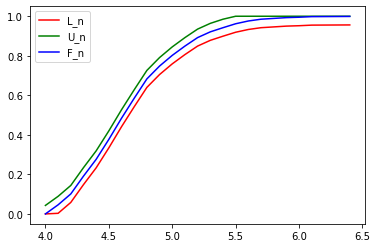
png
# Now to find the confidence interval, using the result from 8.5.6:

import math
from scipy.stats import norm

#ppf(q, loc=0, scale=1) Percent point function (inverse of cdf — percentiles).
#The method norm.ppf() takes a percentage and returns a standard deviation multiplier
#for what value that percentage occurs at.

z_95 = norm.ppf(.975)
theta = F_n(4.9) - F_n(4.3)
se = math.sqrt(theta * (1 - theta) / n)

print('95%% confidence interval: (%.3f, %.3f)' % ((theta - z_95 * se), (theta + z_95 * se)))
95% confidence interval: (0.526, 0.588)Exercise 8.5.8. Get the data on eruption times and waiting times between eruptions of the old faithful geyser from the course website.
- Estimate the mean waiting time and give a standard error for the estimate.
- Also, give a 90% confidence interval for the mean waiting time.
- Now estimate the median waiting time.
In the next chapter we will see how to get the standard error for the median.
import pandas as pd

data = pd.read_csv('data/geysers.csv', sep=',')
r = np.array(data['waiting'])
data| index | eruptions | waiting | |
|---|---|---|---|
| 0 | 1 | 3.600 | 79 |
| 1 | 2 | 1.800 | 54 |
| 2 | 3 | 3.333 | 74 |
| 3 | 4 | 2.283 | 62 |
| 4 | 5 | 4.533 | 85 |
| … | … | … | … |
| 267 | 268 | 4.117 | 81 |
| 268 | 269 | 2.150 | 46 |
| 269 | 270 | 4.417 | 90 |
| 270 | 271 | 1.817 | 46 |
| 271 | 272 | 4.467 | 74 |
272 rows × 3 columns
# Estimate the mean waiting time and give a standard error for the estimate.
theta = r.mean()
se = r.std()

print("Estimated mean: %.3f" % theta)
print("Estimated SE: %.3f" % se)
Estimated mean: 70.897
Estimated SE: 13.570# Also, give a 90% confidence interval for the mean waiting time.
import math
from scipy.stats import norm
z_90 = norm.ppf(.95)
print('90%% confidence interval: (%.3f, %.3f)' % ((theta - z_90 * se), (theta + z_90 * se)))90% confidence interval: (48.576, 93.218)# Now estimate the median time
median = np.median(r)
print("Estimated median time: %.3f" % median)Estimated median time: 76.000Exercise 8.5.9. 100 people are given a standard antibiotic to treat an infection and another 100 are given a new antibiotic. In the first group, 90 people recover; in the second group, 85 people recover. Let \(p_1\) be the probability of recovery under the standard treatment, and let \(p_2\) be the probability of recovery under the new treatment. We are interested in estimating \(\theta = p_1 - p_2\). Provide an estimate, standard error, an 80% confidence interval and a 95% confidence interval for \(\theta\).
Solution. Let \(X_1, \dots, X_100\) be indicator random variables (0 or 1) determining recovery on the first group, and \(Y_1, \dots, Y_100\) indicating recovery on the second group. From the problem formulation, we can assume \(X_i \sim \text{Bernoulli}(p_1)\) and \(Y_i \sim \text{Bernoulli}(p_2)\).
If \(\theta = p_1 - p_2\), then from exercise 8.5.2:
\[\hat{\theta} = \hat{p_1} - \hat{p_2}\]
\[\text{se}(\hat{\theta}) = \sqrt{\hat{p_1}(1 - \hat{p_1}) + \hat{p_2}(1 - \hat{p_2})}\]
import math

p_hat_1 = 0.9
p_hat_2 = 0.85

theta_hat = p_hat_1 - p_hat_2
se_theta_hat = math.sqrt(p_hat_1 * (1 - p_hat_1) + p_hat_2 * (1 - p_hat_2))

print('Estimated mean: %.3f' % theta_hat)
print('Estimated SE: %.3f'   % se_theta_hat)
Estimated mean: 0.050
Estimated SE: 0.466from scipy.stats import norm
z_80 = norm.ppf(.9)
z_95 = norm.ppf(.975)
print('80%% confidence interval: (%.3f, %.3f)' % ((theta_hat - z_80 * se_theta_hat), (theta_hat + z_80 * se_theta_hat)))
print('95%% confidence interval: (%.3f, %.3f)' % ((theta_hat - z_95 * se_theta_hat), (theta_hat + z_95 * se_theta_hat)))80% confidence interval: (-0.548, 0.648)
95% confidence interval: (-0.864, 0.964)Exercise 8.5.10. In 1975, an experiment was conducted to see if cloud seeding produced rainfall. 26 clouds were seeded with silver nitrate and 26 were not. The decision to seed or not was made at random. Get the data from the provided link.
Let \(\theta\) be the difference in the median precipitation from the two groups.
- Estimate \(\theta\).
- Estimate the standard error of the estimate and produce a 95% confidence interval.
import numpy as np
import pandas as pd
from tqdm import notebook

data = pd.read_csv('data/cloud_seeding.csv', sep=',')
X = data['Seeded_Clouds']
Y = data['Unseeded_Clouds']
data| Unseeded_Clouds | Seeded_Clouds | |
|---|---|---|
| 0 | 1202.6 | 2745.6 |
| 1 | 830.1 | 1697.8 |
| 2 | 372.4 | 1656.0 |
| 3 | 345.5 | 978.0 |
| 4 | 321.2 | 703.4 |
| 5 | 244.3 | 489.1 |
| 6 | 163.0 | 430.0 |
| 7 | 147.8 | 334.1 |
| 8 | 95.0 | 302.8 |
| 9 | 87.0 | 274.7 |
| 10 | 81.2 | 274.7 |
| 11 | 68.5 | 255.0 |
| 12 | 47.3 | 242.5 |
| 13 | 41.1 | 200.7 |
| 14 | 36.6 | 198.6 |
| 15 | 29.0 | 129.6 |
| 16 | 28.6 | 119.0 |
| 17 | 26.3 | 118.3 |
| 18 | 26.1 | 115.3 |
| 19 | 24.4 | 92.4 |
| 20 | 21.7 | 40.6 |
| 21 | 17.3 | 32.7 |
| 22 | 11.5 | 31.4 |
| 23 | 4.9 | 17.5 |
| 24 | 4.9 | 7.7 |
| 25 | 1.0 | 4.1 |
theta_hat = X.median() - Y.median()

print('Estimated mean: %.3f' % theta_hat)
Estimated mean: 177.400# Using bootstrap (from chapter 9):
nx = len(X)
ny = len(Y)
B = 10000
t_boot = np.zeros(B)
for i in notebook.tqdm(range(B)):
xx = X.sample(n=nx, replace=True)
yy = Y.sample(n=ny, replace=True)
t_boot[i] = xx.median() - yy.median()
se = np.array(t_boot).std()
print('Estimated SE: %.3f' % se) 0%| | 0/10000 [00:00<?, ?it/s]
Estimated SE: 64.244# See example 9.5, page 135
from scipy.stats import norm
z_95 = norm.ppf(.975)
normal_conf = (theta_hat - z_95 * se, theta_hat + z_95 * se)
percentile_conf = (np.quantile(t_boot, .025), np.quantile(t_boot, .975))
pivotal_conf = (2*theta_hat - np.quantile(t_boot, 0.975), 2*theta_hat - np.quantile(t_boot, .025))
print('95%% confidence interval (Normal): \t %.3f, %.3f' % normal_conf)
print('95%% confidence interval (percentile): \t %.3f, %.3f' % percentile_conf)
print('95%% confidence interval (pivotal): \t %.3f, %.3f' % pivotal_conf)95% confidence interval (Normal): 53.080, 301.720
95% confidence interval (percentile): 37.450, 263.950
95% confidence interval (pivotal): 90.850, 317.350