6. Convergence of Random Variables
6.2 Types of convergence
\(X_n\) converges to \(X\) in probability, written \(X_n \xrightarrow{\text{P}} X\), if, for every \(\epsilon > 0\),:
\[ \mathbb{P}( |X_n - X| > \epsilon ) \rightarrow 0 \]
as \(n \rightarrow \infty\).
\(X_n\) converges to \(X\) in distribution, written \(X_n \leadsto X\), if
\[ \lim _{n \rightarrow \infty} F_n(t) = F(t) \]
for all \(t\) for which \(F\) is continuous.
\(X_n\) converges to \(X\) in quadratic mean, written \(X_n \xrightarrow{\text{qm}} X\), if,
\[ \mathbb{E}(X_n - X)^2 \rightarrow 0 \]
as \(n \rightarrow \infty\).
Theorem 6.4. The following relationships hold:
\(X_n \xrightarrow{\text{qm}} X\) implies that \(X_n \xrightarrow{P} X\).
\(X_n \xrightarrow{\text{P}} X\) implies that \(X_n \leadsto X\).
if \(X_n \leadsto X\) and if \(\mathbb{P}(X = c) = 1\) for some real number \(c\), then \(X_n \xrightarrow{\text{P}} X\).
Proof
- Fix \(\epsilon > 0\). Using Chebyshev’s inequality,
\[ \mathbb{P}(|X_n - X| > \epsilon) = \mathbb{P}(|X_n - X|^2 > \epsilon^2) \leq \frac{\mathbb{E}|X_n - X|^2}{\epsilon^2} \rightarrow 0 \]
- Fix \(\epsilon > 0\) and let \(x\) be a point of continuity of \(F\). Then
\[ \begin{align} F_n(x) & = \mathbb{P}(X_n \leq x) = \mathbb{P}(X_n \leq x, X \leq x + \epsilon) + \mathbb{P}(X_n \leq x, X > x + \epsilon) \\ & \leq \mathbb{P}(X \leq x + \epsilon) + \mathbb{P}(|X_n - X| > \epsilon) \\ & = F(x + \epsilon) + \mathbb{P}(|X_n - X| > \epsilon) \end{align} \]
Also,
\[ \begin{align} F(x - \epsilon) & = \mathbb{P}(X \leq x - \epsilon) = \mathbb{P}(X \leq x - \epsilon, X_n \leq x) + \mathbb{P}(X \leq x + \epsilon, X_n > x) \\ & \leq F_n(x) + \mathbb{P}(|X_n - X| > \epsilon) \end{align} \]
Hence,
\[ F(x - \epsilon) - \mathbb{P}(|X_n - X| > \epsilon) \leq F_n(x) \leq F_n(x + \epsilon) + \mathbb{P}(|X_n - X| > \epsilon) \]
Take the limit as \(n \rightarrow \infty\) to conclude that
\[ F(x - \epsilon) \leq \liminf_{n \rightarrow \infty} F_n(x) \leq \limsup_{n \rightarrow \infty} F_n(x) \leq F(x + \epsilon) \]
- Fix \(\epsilon > 0\). Then,
\[ \begin{align} \mathbb{P}(|X_n - c| > \epsilon) & = \mathbb{P}(X_n < c - \epsilon) + \mathbb{P}(X_n > c + \epsilon) \\ & \leq \mathbb{P}(X_n \leq c - \epsilon) + \mathbb{P}(X_n > c + \epsilon) \\ & = F_n(c - \epsilon) + 1 - F_n(c + \epsilon) \\ & \rightarrow F(c - \epsilon) + 1 - F(c + \epsilon) \\ & = 0 + 1 - 1 = 0 \end{align} \]
Now, to show that the reverse implications do not hold:
Convergence in probability does not imply convergence in quadratic mean
Let \(U \sim \text{Unif}(0, 1)\), and let \(X_n \sim \sqrt{n} I_{(0, 1 / n)}(U)\). Then \(\mathbb{P}(|X_n| > \epsilon) = \mathbb{P}(\sqrt{n} I_{(0, 1 / n)}(U) > \epsilon) = \mathbb{P}(0 \leq U < 1/n) = 1/n \rightarrow 0\). Hence, then \(X_n \xrightarrow{\text{P}} 0\). But \(\mathbb{E}(X_n^2) = n \int_0^{1/n} du = 1\) for all \(n\) so \(X_n\) does not converge in quadratic mean.
Convergence in distribution does not imply convergence in probability
Let \(X \sim N(0, 1)\). Let \(X_n = -X\) for \(n = 1, 2, 3, \dots\); hence \(X_n \sim N(0, 1)\). \(X_n\) has the same distribution as \(X\) for all \(n\) so, trivially, \(\lim _n F_n(x) \rightarrow F(x)\) for all \(x\). Therefore, \(X_n \leadsto X\). But \(\mathbb{P}(|X_n - X| > \epsilon) = \mathbb{P}(|2X| > \epsilon) \neq 0\). So \(X_n\) does not tend to \(X\) in probability.
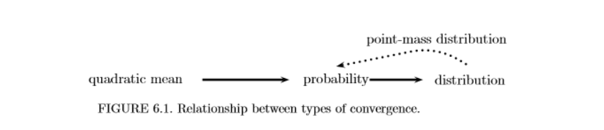
image.png
Theorem 6.5 Let \(X_n, X, Y_n, Y\) be random variables. Let \(g\) be a continuous function. Then:
- If \(X_n \xrightarrow{\text{P}} X\) and \(Y_n \xrightarrow{\text{P}} Y\), then \(X_n + Y_n \xrightarrow{\text{P}} X + Y\).
- If \(X_n \xrightarrow{\text{qm}} X\) and \(Y_n \xrightarrow{\text{qm}} Y\), then \(X_n + Y_n \xrightarrow{\text{qm}} X + Y\).
- If \(X_n \leadsto X\) and \(Y_n \leadsto c\), then \(X_n + Y_n \leadsto X + c\).
- If \(X_n \xrightarrow{\text{P}} X\) and \(Y_n \xrightarrow{\text{P}} Y\), then \(X_n Y_n \xrightarrow{\text{P}} XY\).
- If \(X_n \leadsto X\) and \(Y_n \leadsto c\), then \(X_n Y_n \leadsto cX\).
- If \(X_n \xrightarrow{\text{P}} X\) then \(g(X_n) \xrightarrow{\text{P}} g(X)\) .
- If \(X_n \leadsto X\) then \(g(X_n) \leadsto g(X)\).
6.3 The Law of Large Numbers
Theorem 6.6 (The Weak Law of Large Numbers (WLLN)). If \(X_1, X_2, \dots, X_n\) are IID, then \(\overline{X}_n \xrightarrow{\text{P}} \mu\).
Proof: Assume that \(\sigma < \infty\). This is not necessary but it simplifies the proof. Using Chebyshev’s inequality,
\[ \mathbb{P}(|\overline{X}_n - \mu| > \epsilon) \leq \frac{\mathbb{E}(|\overline{X}_n - \mu|^2)}{\epsilon^2} = \frac{\mathbb{V}(\overline{X}_n)}{\epsilon^2} = \frac{\sigma^2}{n \epsilon^2} \]
which tends to 0 as \(n \rightarrow \infty\).
6.4 The Central Limit Theorem
Theorem 6.8 (The Central Limit Theorem (CLT)). Let \(X_1, X_2, \dots, X_n\) be IID with mean \(\mu\) and variance \(\sigma^2\). Let \(\overline{X}_n = n^{-1}\sum_{i=1}^n X_i\). Then
\[ Z_n \equiv \frac{\sqrt{n} \left( \overline{X}_n - \mu \right)}{\sigma} \leadsto Z \]
where \(Z \sim N(0, 1)\). In other words,
\[ \lim _{n \rightarrow \infty} \mathbb{P}(Z_n \leq z) = \Phi(z) = \int _{-\infty} ^z \frac{1}{\sqrt{2 \pi}} e^{-x^2/2}dx\]
In addition to \(Z_n \leadsto N(0, 1)\), there are several forms of notation to denote the fact that the distribution of \(Z_n\) is converging to a Normal. They all mean the same thing. Here they are:
\[ \begin{align} Z_n & \approx N(0, 1) \\ \overline{X}_n & \approx N\left( \mu, \frac{\sigma^2}{n} \right) \\ \overline{X}_n - \mu & \approx N\left( 0, \frac{\sigma^2}{n} \right) \\ \sqrt{n}(\overline{X}_n - \mu) & \approx N\left( 0, \sigma^2 \right) \\ \frac{\sqrt{n}(\overline{X}_n - \mu)}{\sigma} & \approx N(0, 1) \end{align} \]
The central limit theorem tells us that \(Z_n = \sqrt{n}(\overline{X}_n - \mu)/\sigma\) is approximately \(N(0, 1)\). However, we rarely know \(\sigma\). We can estimate \(\sigma^2\) from \(X_1, X_2, \dots, X_n\) by
\[ S_n^2 = \frac{1}{n - 1} \sum_{i=1}^n ( X_i - \overline{X}_n )^2 \]
This raises the following question: if we replace \(\sigma\) with \(S_n\) is the central limit theorem still true? The answer is yes.
Theorem 6.10. Assume the same conditions as the CLT. Then,
\[ \frac{\sqrt{n} \left(\overline{X}_n - \mu \right)}{S_n} \leadsto N(0, 1)\]
You might wonder how accurate the normal approximation is. The answer is given by the Berry-Essèen theorem.
Theorem 6.11 (Berry-Essèen). Suppose that \(\mathbb{E}|X_1|^3 < \infty\). Then
\[ \sup _z |\mathbb{P}(Z_n \leq z) - \Phi(z)| \leq \frac{33}{4} \frac{\mathbb{E}|X_1 - \mu|^3}{\sqrt{n}\sigma^3} \]
There is also a multivariate version of the central limit theorem.
Theorem 6.12 (Multivariate central limit theorem). Let \(X_1, \dots, X_n\) be IID random vectors where
\[ X_i = \begin{pmatrix} X_{1i} \\ X_{2i} \\ \vdots \\ X_{ki} \end{pmatrix}\]
with mean
\[ \mu = \begin{pmatrix} \mu_1 \\ \mu_2 \\ \vdots \\ \mu_k \end{pmatrix} = \begin{pmatrix} \mathbb{E}(X_{1i}) \\ \mathbb{E}(X_{2i}) \\ \vdots \\ \mathbb{E}(X_{ki}) \end{pmatrix} \]
and variance matrix \(\Sigma\). Let
\[ \overline{X} = \begin{pmatrix} \overline{X}_1 \\ \overline{X}_2 \\ \vdots \\ \overline{X}_k \end{pmatrix}\]
where \[\overline{X}_r = n^{-1}\sum_{i=1}^n X_{ri}\]. Then,
\[ \sqrt{n} (\overline{X} - \mu) \leadsto N(0, \Sigma) \]
6.5 The Delta Method
Theorem 6.13 (The Delta Method). Suppose that
\[ \frac{\sqrt{n}(Y_n - \mu)}{\sigma} \leadsto N(0, 1)\]
and that \(g\) is a differentiable function such that \(g'(u) \neq 0\). Then
\[ \frac{\sqrt{n}(g(Y_n) - g(u))}{|g'(u)| \sigma} \leadsto N(0, 1)\]
In other words,
\[ Y_n \approx N \left( \mu, \frac{\sigma^2}{n} \right) \Rightarrow g(Y_n) \approx N \left( g(\mu), (g'(\mu))^2 \frac{\sigma^2}{n} \right) \]
Theorem 6.15 (The Multivariate Delta method). Suppose that \(Y_n = (Y_{n1}, \dots, Y_{nk})\) is a sequence of random vectors such that
\[ \sqrt{n}(Y_n - \mu) \leadsto N(0, \Sigma) \]
Let \(g : \mathbb{R}^k \rightarrow \mathbb{R}\) and let
\[ \nabla g = \begin{pmatrix} \frac{\partial g}{\partial y_1} \\ \vdots \\ \frac{\partial g}{\partial y_k} \end{pmatrix} \]
Let \(\nabla_\mu\) denote \(\nabla g(y)\) evaluated at \(y = \mu\) and assume that the elements of \(\nabla_\mu\) are non-zero. Then
\[ \sqrt{n}(g(Y_n) - g(\mu)) \leadsto N(0, \nabla_\mu^T \Sigma \nabla_\mu) \]
6.6 Technical appendix
\(X_n\) converges to \(X\) almost surely, written \(X_n \xrightarrow{\text{as}} X\), if
\[ \mathbb{P}(\{s : X_n(s) \rightarrow X(s)\}) = 1 \]
\(X_n\) converges to \(X\) in \(L_1\), written \(X_n \xrightarrow{L_1} X\), if
\[ \mathbb{E} |X_n - X| \rightarrow 0 \]
Theorem 6.17. Let \(X_n\) and \(X\) be random variables. Then:
- \(X_n \xrightarrow{\text{as}} X\) implies that \(X_n \xrightarrow{\text{P}} X\).
- \(X_n \xrightarrow{\text{qm}} X\) implies that \(X_n \xrightarrow{L_1} X\).
- \(X_n \xrightarrow{L_1} X\) implies that \(X_n \xrightarrow{\text{P}} X\).
The weak law of large numbers says that \(\overline{X}_n\) converges to \(\mathbb{E} X\) in probability. The strong law asserts that this is also true almost surely.
Theorem 6.18 (The strong law of large numbers). Let \(X_1, X_2, \dots, X_n\) be IID. If \(\mu = \mathbb{E}|X_1| < \infty\) then \(\overline{X}_n \xrightarrow{\text{as}} \mu\).
A sequence is asymptotically uniformly integrable if
\[ \lim _{M \rightarrow \infty} \limsup _{n \rightarrow \infty} \mathbb{E} ( |X_n| I(|X_n| > M) ) = 0 \]
If \(X_n \xrightarrow{\text{P}} b\) and \(X_n\) is asymptotically uniformly integrable, then \(\mathbb{E}(X_n) \rightarrow b\).
The moment generating function of a random variable \(X\) is
\[\psi_X(t) = \mathbb{E}(e^{tX}) = \int_u e^{tu} f_X(u) du\]
Lemma 6.19. Let \(Z_1, Z_2, \dots, Z_n\) be a sequence of random variables. Let \(\psi_n\) be the mgf of \(Z_n\). Let \(Z\) be another random variable and denote its mgf by \(\psi\). If \(\psi_n(t) \rightarrow \psi(t)\) for all \(t\) in some open interval around 0, then \(Z_n \leadsto Z\).
Proof of the Central Limit Theorem
Let \(Y_i = (X_i - \mu) / \sigma\). Then, \[Z_n = \sqrt{n}(\overline{X}_n - \mu)/\sigma= n^{-1/2} \sum_i Y_i\]. Let \(\psi(t)\) be the mgf of \(Y_i\). The mgf of \(\sum_i Y_i\) is \((\psi(t))^n\) and the mgf of \(Z_n\) is \([\psi(t / \sqrt{n})]^n \equiv \xi_n(t)\).
Now \(\psi'(0) = \mathbb{E}(Y_1) = 0\) and \(\psi''(0) = \mathbb{E}(Y_1^2) = \mathbb{V}(Y_1) = 1\). So,
\[ \begin{align} \psi(t) & = \psi(0) + t \psi'(0) + \frac{t^2}{2!} \psi''(0) + \frac{t^3}{3!} \psi'''(0) + \dots \\ & = 1 + 0 + \frac{t^2}{2} + \frac{t^3}{3!} \psi'''(0) + \ldots \\ & = 1 + \frac{t^2}{2} + \frac{t^3}{3!} \psi'''(0) + \ldots \end{align} \]
Now,
\[ \begin{align} \xi_n(t) & = \left[ \psi \left( \frac{t}{\sqrt{n}} \right) \right] ^n \\ & = \left[ 1 + \frac{t^2}{2n} + \frac{t^3}{3!n^{3/2}} \psi'''(0) + \ldots \right] ^n \\ & = \left[ 1 + \frac{\frac{t^2}{2} + \frac{t^3}{3!n^{1/2}} \psi'''(0) + \ldots}{n} \right] ^n \\ & \rightarrow e^{t^2/2} \end{align} \]
which is the mgf of \(N(0, 1)\). The resolt follows from the previous theorem. In the last step we used the fact that, if \(a_n \rightarrow a\), then
\[ \left( 1 + \frac{a_n}{n} \right) ^n \rightarrow e^a \]
6.8 Exercises
Exercise 6.8.1. Let \(X_1, \dots, X_n\) be iid with finite mean \(\mu = \mathbb{E}(X_i)\) and finite variance \(\sigma^2 = \mathbb{V}(X_i)\). Let \(\overline{X}_n\) be the sample mean and let \(S_n^2\) be the sample variance.
(a) Show that \(\mathbb{E}(S_n^2) = \frac{n-1}{n}\sigma^2\).
Solution:
\(S_n^2\) is the sample variance, that is, $ S_n^2 = n^{-1} _{i=1}^n ( X_i - _n)^2 $. Therefore:
\[ \begin{align} \mathbb{E}[S_n^2] & = \mathbb{E}\left[ \frac 1n \sum_{i=1}^n \left(X_i - \frac 1n \sum_{j=1}^n X_j \right)^2 \right] \\ & = \frac 1n \sum_{i=1}^n \mathbb{E}\left[ X_i^2 - \frac 2n X_i \sum_{j=1}^n X_j + \frac{1}{n^2} \sum_{j=1}^n X_j \sum_{k=1}^n X_k \right] \\ & = \frac 1n \sum_{i=1}^n \left[ \frac{n-2}{n} \mathbb{E}[X_i^2] - \frac{2}{n} \sum_{j \neq i} \mathbb{E}[X_i X_j] + \frac{1}{n^2} \sum_{j=1}^n \sum_{k \neq j}^n \mathbb{E}[X_j X_k] +\frac{1}{n^2} \sum_{j=1}^n \mathbb{E}[X_j^2] \right] \\ & = \frac 1n \sum_{i=1}^n \left[ \frac{n-2}{n} (\sigma^2+\mu^2) - \frac 2n (n-1) \mu^2 + \frac{1}{n^2} n (n-1) \mu^2 + \frac 1n (\sigma^2+\mu^2) \right] \\ & = \frac 1n \sum_{i=1}^n \left[ \frac{n-1}{n} (\sigma^2+\mu^2) - \frac {2}{n} (n-1) \mu^2 + \frac{1}{n} (n-1) \mu^2 \right] \\ & = \frac 1n \sum_{i=1}^n \left[ \frac{n-1}{n} (\sigma^2+\mu^2) - \frac{1}{n} (n-1) \mu^2 \right] \\ & = \frac{n-1}{n} \sigma^2 \end{align} \]
(b) Show that \(S_n^2 \xrightarrow{\text{P}} \sigma^2\).
Hint: show that \(S_n^2 = c_n n^{-1} \sum_{i=1}^n X_i^2 - d_n \overline{X}_n^2\) where \(c_n \rightarrow 1\) and \(d_n \rightarrow 1\). Apply the law of large numbers to \(n^{-1}\sum_{i=1}^n X_i^2\) and to \(\overline{X}_n\). Then use part (e) of Theorem 6.5.
Solution:
We have:
\[ \begin{align} \overline{X}_n^2 & = \frac{1}{n^2} \left( \sum_{i=1}^n X_i \right)^2 \\ &= \frac{1}{n^2} \sum_{i=1}^n X_i^2 + \frac{1}{n^2} \sum_{i=1}^n \sum_{j=1, i \neq j}^n X_i X_j \end{align} \]
Isolating the sum of products, we have:
\[ \sum_{j=1, i \neq j}^n X_i X_j = n^2 \overline{X}_n^2 - \sum_{i=1}^n X_i^2 \]
Now, from the sample variance :
\[ \begin{align} S_n^2 & = \frac{1}{n} \sum_{i=1}^n ( X_i - \overline{X}_n)^2 \\ & = \frac{1}{n} \sum_{i=1}^n \left( X_i^2 - 2 X_i \overline{X}_n + \overline{X}_n^2 \right)\\ & = \frac{1}{n} \sum_{i=1}^n X_i^2 - \overline{X}_n^2\\ \end{align} \]
We can use \(c_n = 1\) and \(d_n = 1\), as suggested in the hint. Applying the law of large numbers,
\[ n^{-1} \sum_{i=1}^n X_i^2 \xrightarrow{\text{P}} n^{-1} \sum_{i=1}^n \mathbb{E}(X_i^2) = \sigma^2 + \mu^2\]
\[ \overline{X}_n \xrightarrow{\text{P}} n^{-1} \sum_{i=1}^n \mathbb{E}(X_i) = \mu \Rightarrow \overline{X}_n^2 \xrightarrow{\text{P}} \mu^2 \]
Therefore, from theorem 6.5.e, $ S_n^2 = c_n n^{-1} _{i=1}^n X_i^2 - d_n _n^2 ^2 + ^2 - ^2 = ^2$.
Exercise 6.8.2. Let \(X_1, X_2, \dots, X_n\) be a sequence of random variables. Show that \(X_n \xrightarrow{\text{qm}} b\) if and only if
\[ \begin{equation} \lim_{n \rightarrow \infty} \mathbb{E}(X_n) = b \quad\mathrm{and}\quad \lim_{n \rightarrow \infty} \mathbb{V}(X_n) = 0 \end{equation} \]
Solution:
\(X_n \xrightarrow{\text{qm}} b\) id equivalent to:
\[ \begin{align} \mathbb{E}[(X_n - b)^2] & \rightarrow 0 \\ \mathbb{E}[X_n^2 - 2b X_n + b^2] & \rightarrow 0 \\ \mathbb{E}[X_n^2] - 2b \mathbb{E}[X_n] + b^2 & \rightarrow 0 \\ \mathbb{V}[X_n] + (\mathbb{E}[X_n])^2 - 2b \mathbb{E}[X_n] + b^2 & \rightarrow 0 \end{align} \]
If \(\lim_{n \rightarrow \infty} \mathbb{V}[X_n] = 0\) and \(\lim_{n \rightarrow \infty} \mathbb{E}[X_n] = b\), then
\[ \begin{align} & \lim_{n \rightarrow \infty} \mathbb{E}[(X_n - b)^2] = \\ & = \lim_{n \rightarrow \infty} \mathbb{V}[X_n] + (\mathbb{E}[X_n])^2 - 2b \mathbb{E}[X_n] + b^2 \\ & = \lim_{n \rightarrow \infty} \mathbb{V}[X_n] + (\lim_{n \rightarrow \infty} \mathbb{E}[X_n])^2 - 2b \lim_{n \rightarrow \infty} \mathbb{E}[X_n] + b^2 \\ &= 0 + b^2 - 2b^2 + b^2 \\ &= 0 \end{align} \]
On the other direction, if \(X_n \xrightarrow{\text{qm}} b\), then
\[ \begin{align} \lim_{n \rightarrow \infty} \mathbb{V}[X_n] + (\lim_{n \rightarrow \infty} \mathbb{E}[X_n])^2 - 2b \lim_{n \rightarrow \infty} \mathbb{E}[X_n] + b^2 &= 0 \\ \lim_{n \rightarrow \infty} \mathbb{V}[X_n] + (\lim_{n \rightarrow \infty} \mathbb{E}[X_n] - b)^2 &= 0 \\ \lim_{n \rightarrow \infty} \mathbb{V}[X_n - b] + \lim_{n \rightarrow \infty} (\mathbb{E}[X_n - b])^2 &= 0 \end{align} \]
Since both terms inside the limits are non-negative, the limits themselves are non-negative. Two non-negative values add up to 0, so they must both be zero, and so we have:
\[ \begin{equation} \lim_{n \rightarrow \infty} \mathbb{E}(Y_n) = 0 \quad\mathrm{and}\quad \lim_{n \rightarrow \infty} \mathbb{V}(Y_n) = 0 \end{equation} \]
or, equivalently,
\[ \begin{equation} \lim_{n \rightarrow \infty} \mathbb{E}(X_n) = b \quad\mathrm{and}\quad \lim_{n \rightarrow \infty} \mathbb{V}(X_n) = 0 \end{equation} \]
Exercise 6.8.3. Let \(X_1, X_2, \dots, X_n\) be iid and let \(\mu = \mathbb{E}(X_i)\). Suppose that variance is finite. Show that \(\overline{X}_n \xrightarrow{\text{qm}} \mu\).
Solution.
Let \(Y_i = X_i - \mu\). It has variance \(\sigma_Y = \sigma\) and mean \(\mu_Y = 0\). We have:
\[ \begin{align} & \mathbb{E}[(\overline{X}_n - \mu)^2] \\ & = \mathbb{E}\left[\left(\frac{1}{n} \sum_{i=1}^n (X_i - \mu) \right)^2\right] \\ & = \frac{1}{n^2} \mathbb{E} \left[ \left(\sum_{i=1}^n Y_i \right)^2 \right] \\ & = \frac{1}{n^2} \left( \sum_{i=1}^n \mathbb{E}[Y_i^2] - \sum_{i=1}^n \sum_{j=1, j \neq i}^n \mathbb{E}[Y_i Y_j] \right) \\ & = \frac{1}{n} \left( (\sigma_Y^2 + \mu_Y^2) - (n-1) \mu_Y^2 \right) \\ & = \frac{\sigma^2}{n} \end{align} \]
Therefore, \[\lim _{n \rightarrow \infty} \mathbb{E}[(\overline{X}_n - \mu)^2] = \lim _{n \rightarrow \infty} \sigma^2 / n = 0\], and so \(\overline{X}_n \xrightarrow{\text{qm}} \mu\).
Exercise 6.8.4. Let \(X_1, X_2, \dots\) be a sequence of random variables such that
\[ \begin{equation} \mathbb{P}\left(X_n = \frac{1}{n}\right) = 1 - \frac{1}{n^2} \quad\mathrm{and}\quad \mathbb{P}\left(X_n = n\right) = \frac{1}{n^2} \end{equation} \]
Does \(X_n\) converge in probability? Doex \(X_n\) converge in quadratic mean?
Solution.
For any distribution \(X\), we have:
\[ \begin{align} & \mathbb{P}( |X_n - X| > \epsilon ) = \\ &= \mathbb{P}\left( |X_n - X| > \epsilon \;\middle|\; X_n = \frac{1}{n} \right)\mathbb{P}\left(X_n = \frac{1}{n}\right) + \mathbb{P}\left( |X_n - X| > \epsilon \;\middle|\; X_n = n \right)\mathbb{P}\left(X_n = n\right) \\ &= \mathbb{P}\left( \middle|\frac{1}{n} - X\middle|\; > \epsilon \right)\left(1 - \frac{1}{n^2} \right) + \mathbb{P}\left( |n - X| > \epsilon \right)\frac{1}{n^2} \end{align} \]
Looking at the limit as \(n \rightarrow \infty\),
\[ \begin{align} & \lim _{n \rightarrow \infty} \mathbb{P}( |X_n - X| > \epsilon ) = \\ & = \lim _{n \rightarrow \infty} \mathbb{P}\left( \middle|\frac{1}{n} - X\middle|\; > \epsilon \right)\left(1 - \frac{1}{n^2} \right) + \lim _{n \rightarrow \infty} \mathbb{P}\left( |n - X| > \epsilon \right)\frac{1}{n^2} \\ & = \lim _{n \rightarrow \infty} \mathbb{P}\left( |X| > \epsilon \right) \end{align} \]
If we set \(X = 0\), the limit above will be zero for any positive \(\epsilon\) – so we have \(X_n \xrightarrow{\text{P}} 0\).
Now, for any quadratic mean potential convergence, we have:
\[ \begin{align} & \mathbb{E}\left[(X_n - X)^2\right] = \\ & = \mathbb{E}\left[(X_n - X)^2 \bigg| X_n = \frac{1}{n} \right] \mathbb{P}\left(X_n = \frac{1}{n}\right) + \mathbb{E}\left[(X_n - X)^2 \big| X_n = n \right] \mathbb{P}\left(X_n = n\right) \\ & = \mathbb{E}\left[\left(X - \frac{1}{n}\right)^2 \right] \left(1 - \frac{1}{n^2}\right) + \mathbb{E}\left[(X - n)^2 \right] \frac{1}{n^2} \\ & = \mathbb{E}\left[X^2 - 2Xn^{-1} + n^{-2} \right] \left(1 - \frac{1}{n^2}\right) + \mathbb{E}\left[X^2 - 2Xn + n^2 \right] \frac{1}{n^2} \\ & = \mathbb{E}\left[X^2\right] + \mathbb{E}\left[X\right] \left(\frac{-2}{n} \left(1 - \frac{1}{n^2} \right) -\frac{2}{n}\right) + \frac{1}{n^2} \left(1 - \frac{1}{n^2} \right) + 1 \\ & = \mathbb{E}\left[X^2\right] - \mathbb{E}\left[X\right] \frac{2}{n} \left( 2 - \frac{1}{n^2} \right) + \frac{1}{n^2} \left(1 - \frac{1}{n^2} \right) + 1 \end{align} \]
Taking the limit as \(n \rightarrow \infty\),
\[ \begin{align} & \lim _{n \rightarrow \infty} \mathbb{E}\left[(X_n - X)^2\right] \\ & = 1 + \lim _{n \rightarrow \infty} \mathbb{E}\left[X^2\right] \\ & = 1 + \mathbb{E}\left[X^2\right] \\ & \geq 1 \end{align} \]
so there is no distribution \(X\) for which this value is 0, and so there is no quadratic mean convergence.
Exercise 6.8.5. Let \(X_1, \dots, X_n \sim \text{Bernoulli}(p)\). Prove that
\[ \begin{equation} \frac{1}{n} \sum_{i=1}^n X_i^2 \xrightarrow{\text{P}} p \quad\mathrm{and}\quad \frac{1}{n} \sum_{i=1}^n X_i^2 \xrightarrow{\text{qm}} p \end{equation} \]
Solution.
Given that quadratic mean convergence implies probability convergence, we only need to prove the second proposition.
Let \(Y_i = X_i^2 - p\). Then:
\[ \begin{align} \mathbb{E}[Y_i] & = \mathbb{E}[X_i^2] - p \\ & = \mathbb{V}[X_i] + \mathbb{E}[X_i]^2 - p \\ & = p(1-p) + p^2 - p \\ & = 0 \\ \mathbb{E}[Y_i^2] & = \mathbb{V}[Y_i] + \mathbb{E}[Y_i]^2 \\ & = \mathbb{V}[X_i^2 - p] + 0^2 \\ & = \mathbb{V}[X_i^2] + 0^2 \\ & = \mathbb{V}[X_i]\\ & = p(1-p) \\ \mathbb{E}[Y_i Y_j] & = \text{(for independent variables)}\\ & = \mathbb{E}[Y_i] \mathbb{E}[Y_j] \\ & = 0 \end{align} \]
\[ \begin{align} & \mathbb{E}\left[\left(\left(\frac{1}{n} \sum_{i=1}^n X_i^2\right) - p\right)^2\right] \\ & = \mathbb{E}\left[\left(\frac{1}{n} \sum_{i=1}^n \left(X_i^2 - p\right)\right)^2\right] \\ & = \frac{1}{n^2} \mathbb{E}\left[\left(\sum_{i=1}^n Y_i\right)^2\right] \\ & = \frac{1}{n^2} \mathbb{E}\left[\sum_{i=1}^n Y_i^2 - \sum_{i=1}^n \sum_{j=1, j \neq i}^n Y_i Y_j\right] \\ & = \frac{1}{n^2} \left( \sum_{i=1}^n \mathbb{E}\left[Y_i^2\right] - \sum_{i=1}^n \sum_{j=1, j \neq i}^n \mathbb{E}\left[ Y_i Y_j \right] \right) \\ & = \frac{p(1-p)}{n} \end{align} \]
So, as \(n \rightarrow \infty\), this expectation goes to 0, and we have quadratic mean convergence.
Exercise 6.8.6. Suppose that the height of men has mean 68 inches and standard deviation 4 inches. We draw 100 men at random. Find (approximately) the probability that the average height of men in our sample will be at least 68 inches.
Solution.
We assume all men’s heights are measurements from iid variables \(X_i\) with mean \(\mu = 68\) and variance \(\sigma^2 = 16\).
We need to approximate \(\mathbb{P}(\overline{X}_{100} > \mu)\). But by the central limit theorem,
\[ \overline{X}_n \approx N\left(\mu, \frac{\sigma^2}{n}\right) \]
so this probability will be approximately \[\mathbb{P}\left(\frac{\sqrt{n}(\overline{X}_n - \mu)}{\sigma} \geq \frac{\sqrt{n}(\mu- \mu)}{\sigma}\right) = \mathbb{P}\left(\frac{\sqrt{n}(\overline{X}_n - \mu)}{\sigma} \geq 0 \right) = P(Z \geq 0) = \frac{1}{2}\]
Exercise 6.8.7. Let \(\lambda_n = 1/n\) for \(n = 1, 2, \dots\). Let \(X_n \sim \text{Poisson}(\lambda_n)\).
(a) Show that \(X_n \xrightarrow{\text{P}} 0\).
Solution.
\[ \mathbb{E}(X_n^2) = \mathbb{V}(X_n) + \mathbb{E}(X_n)^2 = \lambda_n + \lambda_n^2 = 1/n + 1/n^2 \]
This quantity goes to zero as \(n \rightarrow \infty\), so we have \(X_n \xrightarrow{\text{qm}} 0\), which implies \(X_n \xrightarrow{\text{P}} 0\).
(b) Let \(Y_n = n X_n\). Show that \(Y_n \xrightarrow{\text{P}} 0\).
Solution.
\[ \mathbb{E}(Y_n^2) = \mathbb{V}(Y_n) + \mathbb{E}(Y_n)^2 = n^2 \lambda_n + n^2\lambda_n^2 = n+1 \]
so we don’t have a straightforward quadratic mean convergence on \(Y_n\).
We don’t have a straightforward \(L_1\) convergence either:
\[\mathbb{E}(|Y_n|) = \mathbb{E}(Y_n) = n \lambda_n = 1\]
However, we can show that \(Y_n \leadsto 0\):
\[\lim _{n \rightarrow \infty} F_{Y_n}(t) = \lim _{n \rightarrow \infty} F_{X_n}(t / n) = 0 \]
as, when \(n \rightarrow \infty\), the portion of the CDF in the positive neighborhood of 0 shrinks to \(F_{Y_1}(0) = 0\).
We also have a point mass distribution on our target distribution \(Y_\infty = 0\): probability of 1 in point 0, and 0 everywhere else.
Therefore, from theorem 6.4 item c, we have \(Y_n \xrightarrow{\text{P}} 0\).
Exercise 6.8.8. Suppose we have a computer program consisting of \(n = 100\) pages of code. Let \(X_i\) be the number of errors in the \(i\)-th page of code. Suppose that the \(X_i\)’s are Poisson with mean 1 and that they are independent. Let \(Y = \sum_{i=1}^n X_i\) be the total number of errors. Use the central limit theorem to approximate \(\mathbb{P}(Y < 90)\).
Solution. We have \(Y = n \overline{X}_n\), the total being \(n\) times the sample mean. We need to approximate:
We need to approximate \(\mathbb{P}(\overline{X}_{100} < 0.9)\). But by the central limit theorem,
\[ \overline{X}_n \approx N\left(\mu, \frac{\sigma^2}{n}\right) \]
so this probability will be approximately \[ \mathbb{P}\left(\frac{\sqrt{n}(\overline{X}_n - \mu)}{\sigma} < \frac{\sqrt{100}(0.9 - 1)}{1}\right) = \mathbb{P}\left(\frac{\sqrt{n}(\overline{X}_n - \mu)}{\sigma} < -1 \right) = P(Z < -1)\]
Exercise 6.8.9. Suppose that \(\mathbb{P}(X = 1) = \mathbb{P}(X = -1) = 1/2\). Define
\[ \begin{equation} X_n = \begin{cases} X & \text{with probability } 1 - \frac{1}{n}\\ e^n & \text{with probability } \frac{1}{n} \end{cases} \end{equation} \]
Does \(X_n\) converge to \(X\) in probability? Does \(X_n\) converge to \(X\) in distribution? Does \(\mathbb{E}(X - X_n)^2\) converge to 0?
Solution.
For any potential quadratic mean convergence, we’d have:
\[ \begin{align} \mathbb{E}(X - X_n)^2 &= \left(\mathbb{E}(X - X_n \middle| X_n = X)\mathbb{P}(X_n = X) + \mathbb{E}(X - X_n \middle| X_n = e^n)\mathbb{P}(X_n = e^n) \right)^2 \\ & = \left(\mathbb{E}(0)\left(1 - \frac{1}{n} \right) + \mathbb{E}(X - e^n)\frac{1}{n} \right)^2 \\ & = \frac{1}{n^2} \mathbb{E}(X - e^n)^2 \\ & = \frac{1}{n^2} \left( \mathbb{E}(X) - e^n \right)^2 \\ & = \frac{e^{2n}}{n^2} \end{align} \]
which does not converge to 0, so we do not have quadratic mean convergence.
For any potential distribution convergence, \(X_n\) has a point mass distribution, and we can write its CDF \(F_{X_n}\) explicitly as:
\[ \begin{equation} F_{X_n}(t) = \begin{cases} 0 & \text{if } t < -1 \\ \frac{1}{2} \left(1 - \frac{1}{n}\right) & \text{if } -1 \leq t < 1 \\ 1 - \frac{1}{n} & \text{if } 1 \leq t < e^n \\ 1 & \text{if } e^n \leq t \end{cases} \end{equation} \]
On the other hand, the CDF \(F_X\) of the target distribution \(X\) is:
\[ \begin{equation} F_X(t) = \begin{cases} 0 & \text{if } t < -1 \\ \frac{1}{2} & \text{if } -1 \leq t < 1 \\ 1 & \text{if } 1 \leq t \end{cases} \end{equation} \]
We then have:
\[ \begin{equation} F_X(t) - F_{X_n}(t) = \begin{cases} 0 & \text{if } t < -1 \\ \frac{1}{2n} & \text{if } -1 \leq t < 1 \\ \frac{1}{n} & \text{if } 1 \leq t < e^n \\ 0 & \text{if } e^n \leq t \end{cases} \end{equation} \]
so \(0 \leq F_X(t) - F_{X_n}(t) \leq 1/n\), which goes to 0 as \(n \rightarrow \infty\). Therefore \(\lim _{n \rightarrow \infty} F_{X_n}(t) = F_X(t)\), or \(X_n \leadsto X\).
Distribution convergence implies probability convergence, so we also have probability convergence, \(X_n \xrightarrow{\text{P}} X\).
Exercise 6.8.10. Let \(Z \sim N(0, 1)\). Let \(t > 0\).
(a) Show that, for any \(k > 0\),
\[\mathbb{P}(|Z| > t) \leq \frac{\mathbb{E}|Z|^k}{t^k}\]
Solution.
We have:
\[ \begin{align} \mathbb{E}|Z|^k &= \int _{-\infty}^{\infty} |z|^{k}\left( \frac{1}{\sqrt{2\pi}} e^{-z^2/2} \right) dz \\ &= \int _{-\infty}^{0} (-z)^{k}\left( \frac{1}{\sqrt{2\pi}} e^{-z^2/2} \right) dz + \int _{0}^{\infty} z^{k}\left( \frac{1}{\sqrt{2\pi}} e^{-z^2/2} \right) dz \\ &= \left\{ \frac{2}{\pi} \right\}^{1/2} \int _{0}^{\infty} z^k \left( e^{-z^2/2} \right) dz \\ \end{align} \]
For t > 0,
\[ \begin{align} &\mathbb{P}(|Z| > t) = \\ &= 2 \int _t^{\infty} \left( \frac{1}{\sqrt{2\pi}} e^{-z^2/2} \right) dz \\ &= \left\{ \frac{2}{\pi} \right\}^{1/2} \int _t^{\infty} e^{-z^2/2} dz \end{align} \]
Now we need to prove:
\[\int _t^{\infty} e^{-z^2/2} dz \leq \frac{1}{t^k}\int _{0}^{\infty} z^k \left(e^{-z^2/2} \right) dz \]
As the integrands are always positive, we can prove the stronger statement that, for \(k \geq 0\):
\[ \begin{align} \int _t^{\infty} e^{-z^2/2} dz & \leq \frac{1}{t^k}\int _{t}^{\infty} z^k \left( e^{-z^2/2} \right) dz \\ t^k \int _t^{\infty} e^{-z^2/2} dz & \leq \int _{t}^{\infty} z^k \left( e^{-z^2/2} \right) dz \\ 0 & \leq \int _{t}^{\infty} (z^k - t^k) \left( e^{-z^2/2} \right) dz \\ \end{align} \]
But that’s true, since \((z^k - t^k) (z e^{-z^2/2}) \geq 0\) whenever \(z \geq t\). So the given statement follows.
(b) (Mill’s inequality) Show that
\[\mathbb{P}(|Z| > t) \leq \left\{ \frac{2}{\pi} \right\}^{1/2} \frac{e^{-t^2/2}}{t}\]
Hint. Note that \(\mathbb{P}(|Z| > t) = 2\mathbb{P}(Z > t)\). Now write out what \(\mathbb{P}(Z > t)\) means and note that \(x/t > 1\) whenever \(x > t\).
Solution.
The stronger result we proved in (a) was, for \(k \geq 0\),
\[ \mathbb{P}(|Z| > t) = \left\{ \frac{2}{\pi} \right\}^{1/2} \int _t^{\infty} e^{-z^2/2} dz \leq \left\{ \frac{2}{\pi} \right\}^{1/2} \frac{1}{t^k}\int _{t}^{\infty} z^k \left( e^{-z^2/2} \right) dz \]
If we use \(k = 1\), we get:
\[ \mathbb{P}(|Z| > t) \leq \left\{ \frac{2}{\pi} \right\}^{1/2} \frac{1}{t}\int _{t}^{\infty} z e^{-z^2/2} dz = \left\{ \frac{2}{\pi} \right\}^{1/2} \frac{e^{-t^2/2}}{t} \]
which is the desired result.
Exercise 6.8.11. Suppose that \(X_n \sim N(0, 1/n)\) and let \(X\) be a random variable with distribution \(F(x) = 0\) if \(x < 0\) and \(F(x) = 1\) if \(x \geq 0\). Does \(X_n\) converge to \(X\) in probability? Does \(X_n\) converge to \(X\) in distribution?
Solution.
We do not have convergence in distribution: $ F_{X_n}(0) = 1/2$ for any \(n\) (as the normal distribution is symmetric around its mean), so \(\lim _{n \rightarrow \infty} F_{X_n}(0) = 1/2 \neq F_X(0) = 1\).
We do have convergence in probability: for every \(\epsilon > 0\),
\[ \mathbb{P}(|X - X_n| > \epsilon) = \mathbb{P}(|X_n| > \epsilon) = 2 \mathbb{P}(X_n > \epsilon) = 2 (1 - F_{X_n}(\epsilon))\]
so
\[ \lim _{n \rightarrow \infty} \mathbb{P}(|X - X_n| > \epsilon) = 2 (1 - \lim _{n \rightarrow \infty} F_{X_n}(\epsilon)) = 2 (1 - \lim _{n \rightarrow \infty} F_{X_1}(n \epsilon)) = 2 (1 - 1) = 0 \]
Exercise 6.8.12. Let \(X, X_1, X_2, X_3, \cdots\) be random variables that are positive and integer valued. Show that \(X_n \leadsto X\) if and only if
\[ \lim _{n \rightarrow \infty} \mathbb{P}(X_n = k) = \mathbb{P}(X = k) \]
for every integer \(k\).
Solution.
If \(X_n \leadsto X\), then \(\lim _{n \rightarrow \infty} F_{X_n}(k) = F_X(k)\) for every integer \(k\). But since the variables are positive and integer valued,
\[ \begin{equation} \mathbb{P}(X_n = k) = F_{X_n}(k) - F_{X_n}(k - 1) \quad\mathrm{and}\quad \mathbb{P}(X = k) = F_X(k) - F_X(k - 1) \end{equation} \]
Therefore,
\[\begin{align} \lim _{n \rightarrow \infty} \mathbb{P}(X_n = k) &= \lim _{n \rightarrow \infty} F_{X_n}(k) - F_{X_n}(k - 1)\\ &= \lim _{n \rightarrow \infty} F_{X_n}(k) - \lim _{n \rightarrow \infty} F_{X_n}(k - 1)\\ &= F_X(k) - F_X(k - 1)\\ &= \mathbb{P}(X = k)\\ \end{align}\]
On the other direction, if \[\lim _{n \rightarrow \infty} \mathbb{P}(X_n = k) = \mathbb{P}(X = k)\], then
\[ \lim _{n \rightarrow \infty}\left( F_{X_n}(k) - F_{X_n}(k - 1) \right) = F_X(k) - F_X(k - 1) \]
But the variables are positive and integer valued, so \(F_{X_n}(k) = F_X(k) = 0\) for \(k \leq 0\). We can then show that \(\lim _{n \rightarrow \infty} F_{X_n}(k) = F_X(k)\) for every integer valued \(k\) by induction in \(k\):
\[ \lim _{n \rightarrow \infty} \left( F_{X_n}(k) - F_{X_n}(k - 1) \right) = \left( \lim _{n \rightarrow \infty} F_{X_n}(k) \right) - F_X(k - 1) = F_X(k) - F_X(k - 1)\] \[ \Rightarrow \lim _{n \rightarrow \infty} F_{X_n}(k) = F_X(k)\]
Since the result holds for every integer variable \(k\) and the random variables can only take integer values, it must hold for all values, therefore \(X_n \leadsto X\).
Exercise 6.8.13. Let \(Z_1, Z_2, \dots\) be iid random variables with density \(f\). Suppose that \(\mathbb{P}(Z_i > 0) = 1\) and that \(\lambda = \lim _{x \downarrow 0} f(x) > 0\). Let
\[ X_n = n \min \{ Z_1, \dots, Z_n \} \]
Show that \(X_n \leadsto Z\) where \(Z\) has and exponential distribution with mean \(1 / \lambda\).
Solution.
Since \(\mathbb{P}(Z_i > 0) = 1\), the cumulative density functions \(F\) assume value 0 for values up until 0 inclusive.
We have:
\[\mathbb{P}(X_n > x) = \mathbb{P}(n \min\{Z_1, \dots, Z_n\} > x) = \prod _{i=1}^n \mathbb{P}(Z_i > x/n)\]
Expanding the probability based on its density function,
\[\begin{align} \mathbb{P}(X_n > x)&= \prod _{i=1}^n \mathbb{P}(Z_i > x/n)\\ &= \prod _{i=1}^n \int _0^{x/n} f(u) du\\ &= \left(F\left(\frac{x}{n}\right) \right)^n\\ &= \left(F(0) + F'(0)\frac{x}{n} + F''(0)\left(\frac{x}{n}\right)^2\frac{1}{2!} + \cdots \right)^n\\ \end{align}\]
Taking the limit as \(n \rightarrow \infty\),
\[ \lim _{n \rightarrow \infty}\mathbb{P}(X_n > x) = \lim _{n \rightarrow \infty} \left(F(0) + F'(0)\frac{x}{n} + F''(0)\left(\frac{x}{n}\right)^2\frac{1}{2!} + \cdots \right)^n\\ = \lim _{n \rightarrow \infty} \left(F(0) + F'(0)\frac{x}{n} \right)^n = \lim _{n \rightarrow \infty} \left(0 + \lambda\frac{x}{n} \right)^n = e^{-\lambda x} \]
On the other hand, \(\mathbb{P}(Z > x) = e^{-\lambda x}\), so the limit of the CDF complements are the same, and so \(X_n \leadsto Z\).
Exercise 6.8.14. Let \(X_1, \dots, X_n \sim \text{Uniform}(0, 1)\). Let \(Y_n = \overline{X}_n^2\). Find the limiting distribution of \(Y_n\).
Solution.
Let \(F_K(x)\) denote the CDF of random variable \(K\).
The sample mean \(\overline{X}_n\) has a limiting distribution of \(X = 1/2\), by the (strong) law of large numbers.
Then, for \(x \geq 0\),
\[\mathbb{P}(Y_n > x) = \mathbb{P}(\overline{X}_n^2 > x) = \mathbb{P}(\overline{X}_n > x^{1/2})\]
\[F_{Y_n}(x) = F_{\overline{X}_n}(x^{1/2}) \]
Since \(\overline{X}_n \leadsto 1/2\),
\[ \begin{align} \lim _{n \rightarrow \infty} F_{\overline{X}_n}(x) & = F_{1/2}(x) \\ \lim _{n \rightarrow \infty} F_{\overline{X}_n}(x^{1/2}) & = F_{1/2}(x^{1/2}) \\ \lim _{n \rightarrow \infty} F_{Y}(x) & = F_{1/2}(x^{1/2}) \end{align} \]
Therefore, \(Y \leadsto Z\), where \(F_Z(x) = F_{1/2}(x^{1/2})\), that is,
\[ \begin{equation} F_Z(t) = \begin{cases} 0 & \text{if } t^{1/2} < 1/2 \\ 1 & \text{otherwise} \end{cases} = \begin{cases} 0 & \text{if } t < 1/4 \\ 1 & \text{otherwise} \end{cases} \end{equation} \]
so \(Z\) assumes the constant value of \(1/4\), and \(Y \leadsto 1/4\).
Exercise 6.8.15. Let
\[ \begin{pmatrix} X_{11} \\ X_{21} \end{pmatrix}, \; \begin{pmatrix} X_{12} \\ X_{22} \end{pmatrix}, \; \cdots, \; \begin{pmatrix} X_{1n} \\ X_{1n} \end{pmatrix} \]
be iid random vectors with mean \(\mu = (\mu_1, \mu_2)\) and variance \(\Sigma\).
Let
\[ \overline{X}_1 = \frac{1}{n}\sum_{i=1}^n X_{1i}, \; \; \; \overline{X}_2 = \frac{1}{n}\sum_{i=1}^n X_{2i} \]
and define \(Y_n = \overline{X}_1 \big/ \overline{X}_2\). Find the limiting distribution of \(Y_n\).
Solution.
Let \[\overline{X} = n^{-1} \sum_{i=1}^n \begin{pmatrix} X_{1i} \\ X_{2i} \end{pmatrix} = \begin{pmatrix} \overline{X}_1 \\ \overline{X}_2 \end{pmatrix}\].
By the multivariate central limit theorem,
\[ \sqrt{n}(\overline{X} - \mu) \leadsto N(0, \Sigma) \]
Define \(g: \mathbb{R} \times \mathbb{R}_{\neq 0} \rightarrow \mathbb{R}\) as:
\[ g \begin{pmatrix} y_1 \\ y_2 \end{pmatrix} = y_1 / y_2 \]
Then, \(Y_n = g(\overline{X_n})\) in every scenario where \(Y_n\) is defined.
Applying the multivariate delta method,
\[ \nabla g = \begin{pmatrix} \frac{\partial g}{\partial y_1} \\ \frac{\partial g}{\partial y_2} \end{pmatrix} = \begin{pmatrix} \frac{1}{y_2} \\ -\frac{y_1}{y_2^2} \end{pmatrix} \]
Then,
\[ \nabla_\mu = \begin{pmatrix} \frac{1}{\mu_2} \\ -\frac{\mu_1}{\mu_2^2} \end{pmatrix} \]
and so
\[ \begin{align} \sqrt{n}(Y_n - g(\mu)) & \leadsto N(0, \nabla_\mu^T \Sigma \nabla_\mu) \\ Y_n & \leadsto N(\mu_1 / \mu_2, n^{-1/2} \nabla_\mu^T \Sigma \nabla_\mu) \end{align} \]