5. Inequalities
5.1 Markov and Chebyshev Inequalities
Theorem 5.1 (Markov’s Inequality). Let \(X\) be a non-negative random variable and suppose that \(\mathbb{E}(X)\) exists. For any \(t > 0\),
\[ \mathbb{P}(X > t) \leq \frac{\mathbb{E}(X)}{t} \]
Proof.
\[ \mathbb{E}(X) =\int_0^\infty xf(x) dx =\int_0^t xf(x) dx + \int_t^\infty xf(x) dx \geq \int_t^\infty xf(x) dx \geq t \int_t^\infty f(x) dx = t \mathbb{P}(X > t) \]
Theorem 5.2 (Chebyshev’s Inequality). Let \(\mu = \mathbb{E}(X)\) and \(\sigma^2 = \mathbb{V}(X)\). Then,
\[ \mathbb{P}(|X - \mu| \geq t) \leq \frac{\sigma^2}{t^2} \quad \text{and} \quad \mathbb{P}(|Z| \geq k) \leq \frac{1}{k^2} \]
where \(Z = (X - \mu) / \sigma\). In particular, \(\mathbb{P}(|Z| > 2) \leq 1/4\) and \(\mathbb{P}(|Z| > 3) \leq 1/9\).
Proof. We use Markov’s inequality to conclude that
\[ \mathbb{P}(|X - \mu| \geq t) = \mathbb{P}(|X - \mu|^2 \geq t^2) \leq \left(\frac{\mathbb{E}(X - \mu)}{t}\right)^2 = \frac{\sigma^2}{t^2} \]
The second part follows by setting \(t = k \sigma\).
5.2 Hoeffding’s Inequality
Hoeffding’s inequality is similar in spirit to Markov’s inequality but it is a sharper inequality. We present the result here in two parts. The proofs are in the technical appendix.
Theorem 5.4. Let \(Y_1, \dots, Y_n\) be independent observations such that \(\mathbb{E}(Y_i) = 0\) and \(a_i \leq Y_i \leq b_i\). Let \(\epsilon > 0\). Then, for any \(t > 0\),
\[ \mathbb{P}\left( \sum_{i=1}^n Y_i \geq \epsilon \right) \leq e^{-t\epsilon} \prod_{i=1}^n e^{t^2(b_i - a_i)^2 / 8} \]
Theorem 5.5. Let \(X_1, \dots, X_n \sim \text{Bernoulli}(p)\). Then, for any \(\epsilon > 0\),
\[ \mathbb{P}(|\overline{X}_n - p| > \epsilon) \leq 2e^{-2n\epsilon^2} \]
Hoeffding’s inequality gives us a simple way go create a confidence interval for a binomial parameter \(p\). We will discuss confidence intervals later but here is the basic idea. Let \(\alpha > 0\) and let
\[ \epsilon_n = \left\{ \frac{1}{2n} \log \left( \frac{2}{\alpha} \right) \right\}^{1/2} \]
By Hoeffding’s inequality,
\[ \mathbb{P}(|\overline{X}_n - p| > \epsilon_n) \leq 2e^{-2n\epsilon_n^2} = \alpha \]
Let \(C = (\overline{X}_n - \epsilon, \overline{X}_n + \epsilon)\). Then, \(\mathbb{P}(\text{not } C \in p) = \mathbb{P}(|\overline{X}_n - p| > \epsilon) \leq \alpha\). Hence, \(\mathbb{P}(p \in C) \geq 1 - \alpha\), that is, ratio \((1 - \alpha)\) of the random intervals \(C\) trap the true parameter \(p\); we call \(C\) a \(1 - \alpha\) confidence interval. More on this later.
5.3 Cauchy-Schwartz and Jensen Inequalities
This section contains two inequalities on expected values that are often useful.
Theorem 5.7 (Cauchy-Schwartz Inequalities). If \(X\) and \(Y\) have finite variances then
\[ \mathbb{E}|XY| \leq \sqrt{\mathbb{E}\left(X^2\right) \mathbb{E}\left(Y^2\right)} \]
Recall that a function \(g\) is convex if for each \(x, y\) and each \(\alpha \in [0, 1]\),
\[ g(\alpha x + (1 - \alpha)y) \leq \alpha g(x) + (1 - \alpha) g(y) \]
If \(g\) is twice differentiable, then the convexity reduces to checking that \(g''(x) \geq 0\) for all \(x\). It can be shown that if \(g\) is convex then it lies above any line that touches \(g\) at some point, called a tangent line. A function \(g\) is concave if \(-g\) is convex. Examples of convex functions are \(g(x) = -x^2\) and \(g(x) = \log x\).
Theorem 5.8 (Jensen’s Inequality). If \(g\) is convex then
\[ \mathbb{E}g(X) \geq g(\mathbb{E}X) \]
If \(g\) is concave then
\[ \mathbb{E}g(X) \leq g(\mathbb{E}X) \]
Proof. Let \(L(x) = a + bx\) be a line, tangent to the \(g(x)\) at the point \(\mathbb{E}(X)\). Since \(g\) is convex, it lies above the line \(L(x)\). So,
\[ \mathbb{E}g(X) \geq \mathbb{E}L(X) = \mathbb{E}(a + bX) = a + b\mathbb{E}(X) = L(\mathbb{E}(X)) = g(\mathbb{E}(X))\]
From Jensen’s inequality we see that \(\mathbb{E}X^2 \geq (\mathbb{E}X)^2\) and \(\mathbb{E}(1/X) \geq 1 / \mathbb{E}(X)\). Since log is concave, \(\mathbb{E}(\log X) \leq \log \mathbb{E}(X)\). For example, suppose that \(X \sim N(3, 1)\). Then \(\mathbb{E}(1 / X) \geq 1/3\).
5.4 Technical Appendix: Proof of Hoeffding’s Inequality
We will make use of the exact form of Taylor’s theorem: if \(g\) is a smooth function, then there is a number \(\xi \in (0, u)\) such that \(g(u) = g(0) + u g'(0) + \frac{u^2}{2}g''(\xi)\).
Proof of Theorem 5.4. For any \(t > 0\), we have, from Markov’s inequality, that
\[ \mathbb{P}\left( \sum_{i=1}^n Y_i \geq \epsilon \right) = \mathbb{P}\left( t \sum_{i=1}^n Y_i \geq t \epsilon \right) = \mathbb{P}\left( e^{t \sum_{i=1}^n Y_i} \geq e^{t \epsilon} \right) \leq e^{-t\epsilon} \mathbb{E}\left( e^{t \sum_{i=1}^n Y_i}\right) = e^{-t\epsilon} \prod_i \mathbb{E}\left(e^{tY_i}\right) \]
Since \(a_i \leq Y_i \leq b_i\), we can write \(Y_i\) as a convex combination of \(a_i\) and \(b_i\), namely, \(Y-i = \alpha b_i + (1 - \alpha) a_i\) where \(\alpha = (Y_i - a_i) / (b_i - a_i)\). So, by the convexity of \(e^{ty}\) we have
\[ e^{tY_i} \leq \frac{Y_i - a_i}{b_i - a_i} e^{tb_i} + \frac{b_i - Y_i}{b_i - a_i} e^{ta_i} \]
Take expectations of both sides and use the fact that \(\mathbb{E}(Y_i) = 0\) to get
\[ \mathbb{E}e^{tY_i} \leq - \frac{a_i}{b_i - a_i} e^{tb_i} + \frac{b_i}{b_i - a_i} e^{ta_i} = e^{g(u)} \]
where \(u = t(b_i - a_i)\), \(g(u) = -\gamma u + \log (1 - \gamma + \gamma e^u)\) and \(\gamma = -a_i / (b_i - a_i)\).
Note that \(g(0) = g'(0) = 0\). Also, \(g''(u) \leq 1/4\) for all \(u > 0\). By Taylor’s theorem, there is a \(\xi \in (0, u)\) such that
\[ g(u) = g(0) + u g'(0) + \frac{u^2}{2} g(\xi) = \frac{u^2}{2} g(\xi) \leq \frac{u^2}{8} = \frac{t^2(b_i - a_i)^2}{8} \]
Hence,
\[ \mathbb{E}e^{tY_i} \leq e^{g(u)} \leq e^{t^2(b_i - a_i)^2/8} \]
and the result follows.
Proof of Theorem 5.5. Let \(Y_i = (1 / n)(X_i - p)\). Then \(\mathbb{E}(Y_i) = 0\) and \(a \leq Y_i \leq b\) where \(a = -p/n\) and \(b = (1 - p) / n\). Also, \((b - a)^2 = 1/n^2\). Applying Theorem 5.4 we get
\[ \mathbb{P}\left(\overline{X}_n - p > \epsilon\right) = \mathbb{P}\left( \sum_i Y_i > \epsilon \right) \leq e^{-t\epsilon} e^{t^2/(8n^2)}\]
The above holds for any \(t > 0\). In particular, take \(t = 4n\epsilon\) and we get \(\mathbb{P}\left(\overline{X}_n - p > \epsilon\right) \leq e^{-2n\epsilon^2}\). By a similar argument we can show that \(\mathbb{P}\left(\overline{X}_n - p < \epsilon\right) \leq e^{-2n\epsilon^2}\). Putting those together we get \(\mathbb{P}\left(|\overline{X}_n - p| > \epsilon\right) \leq 2e^{-2n\epsilon^2}\).
5.6 Exercises
Exercise 5.6.1. Let \(X \sim \text{Exponential}(\beta)\). Find \(\mathbb{P}(|X - \mu_X| > k \sigma_X)\) for \(k > 1\). Compare this to the bound you get from Chebyshev’s inequality.
Solution.
\[ f(x) = \frac{1}{\beta} e^{-x / \beta}, \quad x > 0 \]
Let \(F\) be the CDF of \(X\). We have:
\[ F(x) = \int_{0}^x f(t) dt = \int_{0}^x \frac{1}{\beta} e^{-t / \beta} dt = \frac{1}{\beta} \beta \left( 1 - e^{-x / \beta} \right) = 1 - e^{-x / \beta} \]
We have:
\[ \mathbb{E}(X) = \int_0^\infty x \frac{1}{\beta} e^{-x / \beta} dx = \frac{1}{\beta} \int_0^\infty x e^{-x / \beta} dx = \frac{1}{\beta} \beta^2 = \beta\] \[\mathbb{E}(X^2) = \int_0^\infty x^2 \frac{1}{\beta} e^{-x / \beta} dx = \frac{1}{\beta} \int_0^\infty x^2 e^{-x / \beta} dx = \frac{1}{\beta} 2\beta^3 = 2 \beta^2 \] \[ \mathbb{V}(X) = \mathbb{E}(X^2) - \mathbb{E}(X)^2 = 2\beta^2 - \beta^2 = \beta^2\] and \[\mu_X=\sigma_X=\beta\]
\[ \begin{align} \mathbb{P}(|X - \mu_X| > k \sigma_X) &= 1 - \mathbb{P}(-k \sigma_X < X - \mu_X < k \sigma_X) \\ &= 1 - \mathbb{P}(\mu_X - k \sigma_X < X < \mu_X + k \sigma_X) \\ &= 1 - F(\mu_X + k \sigma_X) + F(\mu_X - k \sigma_X) \\ &= 1 - 1 + \exp\left\{ -\frac{\left(\beta + k \beta\right)^+}{\beta} \right\} + 1 - \exp\left\{-\frac{\left(\beta - k \beta\right)^+}{\beta} \right\} \\ &= 1 + e^{-(1+k)^+ } - e^{-(1-k)^+} \end{align} \]
where \((a)^+ = \max \{ a, 0 \}\).
On the other hand, Chebyshev’s bound provides, for \(t = k\sigma_X\),
\[ \mathbb{P}(|X - \mu_X| \geq k \sigma_X) \leq \frac{\sigma_X^2}{k^2 \sigma_X^2} = \frac{1}{k^2} \]
which is a weaker bound.
import numpy as np
import matplotlib.pyplot as plt
%matplotlib inline

def f(k):
    return 1 + np.exp(-np.maximum(1+k, 0)) - np.exp(-np.maximum(1 - k, 0))

def chebyshev(k):
    # Limit upper bound to 1, since probability is always under 1
    return np.minimum(1 / (k**2), 1)

kk = np.arange(0.01, 10, step = 0.01)

plt.figure(figsize=(12, 8))

plt.plot(kk, f(kk), label='Calculated probability')
plt.plot(kk, chebyshev(kk), label='min(Chebyshev bound, 1)')
plt.yscale('log')
plt.xlabel('k')
plt.ylabel('Probability bound')
plt.legend(loc='lower left')
plt.show()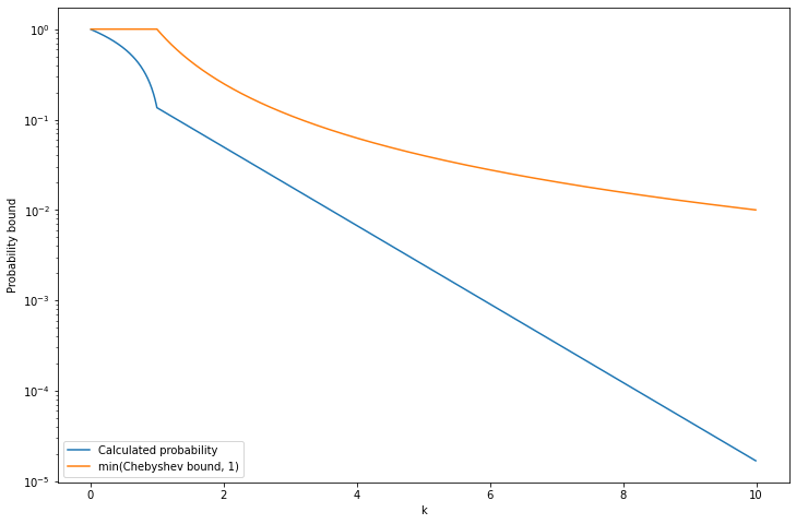
png
Exercise 5.6.2. Let \(X \sim \text{Poisson}(\lambda)\). Use Chebyshev’s inequality to show that \(\mathbb{P}(X \geq 2\lambda) \leq 1 / \lambda\).
Solution. We have \(\mu_X = \lambda\) and \(\sigma_X^2 = \lambda\), so Chebyshev’s gives us:
\[ \mathbb{P}(|X - \lambda| \geq t) \leq \frac{\lambda}{t^2} \]
If we make \(t = \lambda\), we get
\[ \mathbb{P}(X \geq \lambda) = \mathbb{P}(|X - \lambda| \geq \lambda) \leq \frac{1}{\lambda} \]
Exercise 5.6.3. Let \(X_1, \dots, X_n \sim \text{Bernoulli}(p)\) and \(\overline{X}_n = n^{-1} \sum_{i=1}^n X_i\). Bound \(\mathbb{P}(|\overline{X}_n - p| > \epsilon)\) using Chebyshev’s inequality and using Hoeffding’s inequality.
Show that, when \(n\) is large, the bound from Hoeffding’s inequality is smaller than the bound from Chebyshev’s inequality.
Solution. Note that \(\mathbb{E}(\overline{X}_n) = p\) and \(\mathbb{V}(\overline{X}_n) = p(1-p) / n\), since \(n \overline{X}_n \sim \text{Binomial}(n, p)\).
Using Chebyshev’s inequality,
\[ \mathbb{P}(|\overline{X}_n - p| \geq \epsilon) \leq \frac{p(1 - p)}{n \epsilon^2} \]
Using Hoeffding’s inequality,
\[ \mathbb{P}(|\overline{X}_n - p| > \epsilon) \leq 2e^{-2n\epsilon^2} \]
The bound provided by Hoeffding’s inequality is \(O(e^{-2n\epsilon^2})\), while the bound provided by Chebyshev’s inequality is \(O(n^{-1})\), therefore the bound from Hoeffding’s inequality is smaller for a sufficiently large \(n\).
Exercise 5.6.4. Let \(X_1, \dots, X_n \sim \text{Bernoulli}(p)\).
(a) Let \(\alpha > 0\) be fixed and define
\[ \epsilon_n = \sqrt{\frac{1}{2n} \log \left( \frac{2}{\alpha}\right)} \]
Let \(\hat{p}_n = n^{-1} \sum_{i=1}^n X_i\). Define \(C_n = (\hat{p}_n - \epsilon_n, \hat{p}_n + \epsilon_n)\). Use Hoeffding’s inequality to show that
\[ \mathbb{P}(p \in C_n) \geq 1 - \alpha \]
We call \(C_n\) a \(1 - \alpha\) confidence interval for \(p\). In practice, we truncate the interval so it does not go below 0 or above 1.
(b) (Computer Experiment) Let’s examine the properties of this confidence interval. Let \(\alpha = 0.05\) and \(p = 0.4\). Conduct a simulation study to see how often the interval contains \(p\) (called the coverage). Do this for various values of \(n\) between 1 and 10000. Plot the coverage versus \(n\).
(c) Plot the length of the interval versus \(n\). Suppose we want the length of the interval to be no more than .05. How large should \(n\) be?
Solution.
(a) The result is immediate from replacing \(\epsilon_n\) into Hoeffding’s inequality,
\[ \mathbb{P}(|\hat{p}_n - p| > \epsilon_n) \leq 2e^{-2n\epsilon_n^2} = \alpha \]
since \(\mathbb{E}(\hat{p}_n) = p\).
(b)
import numpy as np
from scipy.stats import bernoulli
import tqdm

alpha = 0.05
p = 0.4

B = 50000
N = 10000

nn = np.arange(1, N + 1)
epsilon_n = np.sqrt((1 / (2 * nn)) * np.log(2 / alpha))

p_hat = np.empty((B, N))
for i in tqdm.notebook.tqdm(range(B)):
    X = bernoulli.rvs(p, size=N, random_state=i)
    p_hat[i] = np.cumsum(X) / nn

coverage = np.mean((p_hat + epsilon_n >= p) & (p_hat - epsilon_n <= p), axis=0)
0%| | 0/50000 [00:00<?, ?it/s]import matplotlib.pyplot as plt
%matplotlib inline
plt.figure(figsize=(12, 8))
plt.plot(nn, coverage)
plt.xlabel('n')
plt.ylabel('Coverage')
plt.show()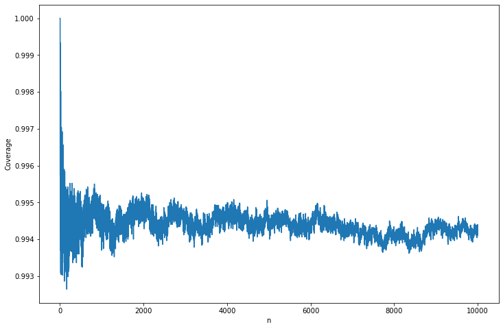
png
(c) The length of the interval is \(\min \{\hat{p}_n + \epsilon_n, 1 \} - \max \{ \hat{p}_n - \epsilon_n, 0\}\). As \(\hat{p}_n \rightarrow p\), let’s plot the approximation on the limit case, which is just \(2 \epsilon_n\).
plt.figure(figsize=(12, 8))
plt.plot(nn, 2 * epsilon_n, label='Interval length')
plt.xlabel('n')
plt.ylabel(r'$2\epsilon_n$')
plt.hlines(.05, xmin=0, xmax=N, color='red', label='Threshold')
plt.yscale('log')
plt.legend(loc='upper right')
plt.show()

selected_n = nn[np.argmax(2 * epsilon_n <= .05)]
print('Smallest n with interval length under .05: %i' % selected_n)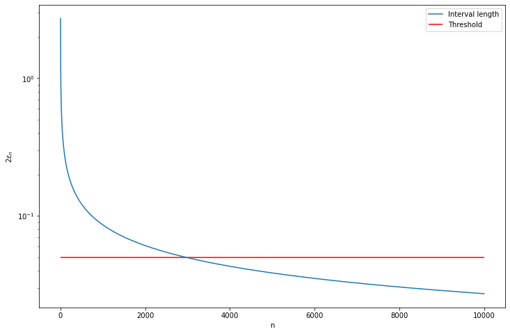
png
Smallest n with interval length under .05: 2952