- 3. Random Variables
- 3.1 Introduction
- 3.2 Distribution Functions and Probability Functions
- 3.3 Some Important Discrete Random Variables
- 3.4 Some Important Continuous Random Variables
- 3.5 Bivariate Distributions
- 3.6 Marginal Distributions
- 3.7 Independent Random Variables
- 3.8 Conditional Distributions
- 3.9 Multivariate Distributions and IID Samples
- 3.10 Two Important Multivariate Distributions
- 3.11 Transformations of Random Variables
- 3.12 Transformation of Several Random Variables
- 3.13 Technical Appendix
- 3.14 Exercises
- References
3. Random Variables
3.1 Introduction
A random variable is a mapping \(X : \Omega \rightarrow \mathbb{R}\) that assigns a real number \(X(\omega)\) to each outcome \(\omega\).
Technically, a random variable must be measurable. See the technical appendix for details.
Given a random variable \(X\) and a subset \(A\) of the real line, define \(X^{-1}(A) = \{ \omega \in \Omega : X(\omega) \in A \}\) and let
\[ \begin{align} \mathbb{P}(X \in A) = \mathbb{P}(X^{-1}(A)) &= \mathbb{P}(\{ \omega \in \Omega; X(\omega) \in A \}) \\ \mathbb{P}(X = x) = \mathbb{P}(X^{-1}(x)) &= \mathbb{P}(\{ \omega \in \Omega; X(\omega) = x \} ) \end{align} \]
\(X\) denotes a random variable and \(x\) denotes a possible value of \(X\).
3.2 Distribution Functions and Probability Functions
The cumulative distribution function, CDF, \(F_X : \mathbb{R} \rightarrow [0, 1]\) of a random variable \(X\) is defined by
\[ F_X(x) = \mathbb{P}(X \leq x) \]
The following result shows that the CDF completely determines the distribution of a random variable.
Theorem 3.7. Let \(X\) have CDF \(F\) and let \(Y\) have CDF \(G\). If \(F(x) = G(x)\) for all \(x\) then \(\mathbb{P}(X \in A) = \mathbb{P}(Y \in A)\) for all \(A\).
Technically, we only have that \(\mathbb{P}(X \in A) = \mathbb{P}(Y \in A)\) for every measurable event \(A\).
Theorem 3.8. A function \(F\) mapping the real line to \([0, 1]\) is a CDF for some probability measure \(\mathbb{P}\) if and only if if satisfies the following three conditions:
- \(F\) is non-decreasing, i.e. \(x_1 < x_2\) implies that \(F(x_1) \leq F(x_2)\).
- \(F\) is normalized: \(\lim_{n \rightarrow -\infty} F(x) = 0\) and \(\lim_{n \rightarrow +\infty} F(x) = 1\).
- \(F\) is right-continuous, i.e. \(F(x) = F(x^+)\) for all \(x\), where
\[ F(x^+) = \lim_{y \rightarrow x, y > x} F(y) \]
Proof. Suppose that \(F\) is a CDF. Let us show that \(F\) is right-continuous. Let \(x\) be a real number and let \(y_1, y_2, \dots\) be a sequence of real numbers such that \(y_1 > y_2 > \dots\) and \(\lim_i y_i = x\). Let \(A_i = (-\infty, y_i]\) and let \(A = (-\infty, x]\). Note that \(A = \cap_{i=1}^\infty A_i\) and also note that \(A_1 \supset A_2 \supset \cdots\). Because the events are monotone, \(\lim_i \mathbb{P}(A_i) = \mathbb{P}(\cap_i A_i)\). Thus,
\[ F(x) = \mathbb{P}(A) = \mathbb{P}(\cap_i A_i) = \lim_i \mathbb{P}(A_i) = \lim_i F(y_i) = F(x^+) \]
Showing that \(F\) is non-decreasing and is normalized is similar. Proving the other direction, that is that \(F\) is non-decreasing, normalized, and right-continuous then it is a CDF for some random variable, uses some deep tools in analysis.
\(X\) is discrete if it takes countably many values
\[ \{ x_1, x_2, \dots \} \]
We define the probability density function or probability mass function for \(X\) by
\[ f_X(x) = \mathbb{P}(X = x) \]
A set is countable if it is finite or if it can be put in a one-to-one correspondence with the integers.
Thus, \(f_X(x) \geq 0\) for all \(x \in \mathbb{R}\) and \(\sum_i f_X(x_i) = 1\). The CDF of \(X\) is related to the PDF by
\[ F_X(x) = \mathbb{P}(X \leq x) = \sum_{x_i \leq x} f_X(x_i) \]
Sometimes we write \(f_X\) and \(F_X\) simply as \(f\) and \(F\).
A random variable \(X\) is continuous if there exists a function \(f_X\) such that \(f_X(x) \geq 0\) for all \(x\), \(\int_{-\infty}^\infty f_X(x) dx = 1\), and for every \(a \leq b\),
\[ \mathbb{P}(a < X < b) = \int_a^b f_X(x) dx \]
The function \(f_X\) is called the probability density function. We have that
\[ F_X(x) = \int_{-\infty}^x f_X(t) dt \]
and \(f_X(x) = F'_X(x)\) at all points \(x\) at which \(F_X\) is differentiable.
Sometimes we shall write \(\int f(x) dx\) or simply \(\int f\) to mean \(\int_{-\infty}^\infty f(x) dx\).
Warning: Note that if \(X\) is continuous then \(\mathbb{P}(X = x) = 0\) for every \(x\). We only have \(f(x) = \mathbb{P}(X = x)\) for discrete random variables; we get probabilities from a PDF by integrating.
Lemma 3.15. Let \(F\) be the CDF for a random variable \(X\). Then:
\(\mathbb{P}(X = x) = F(x) - F(x^-)\) where \(F(x^-) = \lim_{y \uparrow x} F(y)\)
\(\mathbb{P}(x < X \leq y) = F(y) - F(x)\)
\(\mathbb{P}(X > x) = 1 - F(x)\)
If \(X\) is continuous then
\[ \mathbb{P}(a < X < b) = \mathbb{P}(a \leq X < b) = \mathbb{P}(a < X \leq b) = \mathbb{P}(a \leq X \leq b) \]
It is also useful to define the inverse CDF (or quantile function).
Let \(X\) be a random variable with CDF \(F\). The inverse CDF or quantile function is defined by
\[ F^{-1}(q) = \inf \{ x : F(x) \leq q \} \]
for \(q \in [0, 1]\). If \(F\) is strictly increasing and continuous then \(F^{-1}(q)\) is the unique real number \(x\) such that \(F(x) = q\).
We call \(F^{-1}(1/4)\) the first quartile, \(F^{-1}(1/2)\) the median (or second quartile), and \(F^{-1}(3/4)\) the third quartile.
Two random variables \(X\) and \(Y\) are equal in distribution – written \(X \overset{d}= Y\) – if \(F_X(x) = F_Y(x)\) for all \(x\). This does not mean that \(X\) and \(Y\) are equal. Rather, it means that probability statements about \(X\) and \(Y\) will be the same.
3.3 Some Important Discrete Random Variables
Warning about notation: It is traditional to write \(X \sim F\) to indicate that \(X\) has distribution \(F\). This is an unfortunate notation since the symbol \(\sim\) is also used to denote an approximation. The notation is so pervasive we are stuck with it.
.. and we use \(A \approx B\) to denote approximation. The LaTeX macros hint at this common usage: \sim for \(\sim\), and \approx for \(\approx\).
The Point Mass Distribution
\(X\) has a point mass distribution at \(a\), written \(X \sim \delta_a\), if \(\mathbb{P}(X = a) = 1\), in which case
\[ F(x) = \begin{cases} 0 &\text{if } x < a \\ 1 &\text{if } x \geq a \end{cases} \]
The probability mass function is \(f(x) = I(x = a)\), which takes value 1 if \(x = a\) and 0 otherwise.
The Discrete Uniform Distribution
Let \(k > 1\) be a given integer. Suppose that \(X\) has probability mass function given by
\[ f(x) = \begin{cases} 1/k &\text{for } x = 1, \dots, k \\ 0 &\text{otherwise} \end{cases} \]
We say that \(X\) has a uniform distribution on \(\{ 1, \dots, k \}\).
The Bernoulli Distribution
Let \(X\) represent a coin flip. Then \(\mathbb{P}(X = 1) = p\) and \(\mathbb{P}(X = 0) = 1 - p\) for some \(p \in [0, 1]\). We say that \(X\) has a Bernoulli distribution, written \(X \sim \text{Bernoulli}(p)\). The probability mass function is \(f(x) = p^x (1 - p)^{1 - x}\) for \(x \in \{ 0, 1 \}\).
The Binomial Distribution
Suppose we have a coin which falls heads with probability \(p\) for some \(0 \leq p \leq 1\). Flip the coin \(n\) times and let \(X\) be the number of heads. Assume that the tosses are independent. Let \(f(x) = \mathbb{P}(X = x)\) be the mass function. It can be shown that
\[ f(x) = \begin{cases} \binom{n}{x} p^x (1 - p)^{n - x} &\text{for } x= 0, \dots, n \\ 0 &\text{otherwise} \end{cases} \]
A random variable with this mass function is called a Binomial random variable, and we write \(X \sim \text{Binomial}(n, p)\). If \(X_1 \sim \text{Binomial}(n, p_1)\) and \(X_2 \sim \text{Binomial}(n, p_2)\) then \(X_1 + X_2 \sim \text{Bimomial}(n, p_1 + p_2)\).
Note that \(X\) is a random variable, \(x\) denotes a particular value of the random variable, and \(n\) and \(p\) are parameters, that is, fixed real numbers.
The Geometric Distribution
\(X\) has a geometric distribution with parameter \(p \in (0, 1)\), written \(X \sim \text{Geom}(p)\), if
\[\mathbb{P}(X = k) = p(1 - p)^{k - 1}, \quad k \geq 1\]
We have that
\[ \sum_{k=1}^\infty \mathbb{P}(X = k) = p \sum_{k=1}^\infty (1 - p)^k = \frac{p}{1 - (1 - p)} = 1 \]
Think of \(X\) as the number of flips needed until the first heads when flipping a coin.
The Poisson Distribution
\(X\) has a Poisson distribution with parameter \(\lambda\), written \(X \sim \text{Poisson}(\lambda)\), if
\[ f(x) = e^{-\lambda} \frac{\lambda^x}{x!}, \quad x \geq 0 \]
Note that
\[ \sum_{x=0}^\infty f(x) = e^{-\lambda} \sum_{x=0}^\infty \frac{\lambda^x}{x!} = e^{-\lambda} e^\lambda = 1 \]
The Poisson distribution is often used as a model for counts of rare events like radioactive decay and traffic accidents. If \(X_1 \sim \text{Poisson}(n, \lambda_1)\) and \(X_2 \sim \text{Poisson}(n, \lambda_2)\) then \(X_1 + X_2 \sim \text{Poisson}(n, \lambda_1 + \lambda_2)\).
Warning: We defined random variables to be mappings from a sample space \(\Omega\) to \(\mathbb{R}\) but we did not mention sample space in any of the distributions above. Let’s construct a sample space explicitly for a Bernoulli random variable. Let \(\Omega = [0, 1]\), and define \(\mathbb{P}\) to satisfy \(\mathbb{P}([a, b]) = b - a\) for \(0 \leq a \leq b \leq 1\). Fix \(p \in [0, 1]\) and define
\[ X(\omega) = \begin{cases} 1 &\text{if }\omega \leq p \\ 0 &\text{if }\omega > p \end{cases} \]
Then \(\mathbb{P}(X = 1) = \mathbb{P}(\omega \leq p) = \mathbb{P}([0, p]) = p\) and \(\mathbb{P}(X = 0) = 1 - p\). Thus, \(X \sim \text{Bernoulli}(p)\). We could do this for all of the distributions defined above. In practice, we think of a random variable like a random number but formally it is a mapping defined on some sample space.
3.4 Some Important Continuous Random Variables
The Uniform Distribution
\(X\) has a uniform distribution with parameters \(a\) and \(b\), written \(X \sim \text{Uniform}(a, b)\), if
\[ f(x) = \begin{cases} \frac{1}{b - a} &\text{for } x \in [a, b] \\ 0 &\text{otherwise} \end{cases}\]
where \(a < b\). The CDF is
\[ F(x) = \begin{cases} 0 &\text{if } x < a \\ \frac{x - a}{b - a} &\text{if } x \in [a, b] \\ 1 &\text{if } x > b \end{cases} \]
Normal (Gaussian)
\(X\) has a Normal (or Gaussian) distribution with parameters \(\mu\) and \(\sigma\), denoted by \(X \sim N(\mu, \sigma^2)\), if
\[ f(x) = \frac{1}{\sigma \sqrt{2 \pi}} \exp \left\{ -\frac{1}{2} \left( \frac{x - \mu}{\sigma} \right)^2\right\}, \quad x \in \mathbb{R} \]
where \(\mu \in \mathbb{R}\) and \(\sigma > 0\). Later we shall see that \(\mu\) is the “center” (or mean) of the distribution and that \(\sigma\) is the “spread” (or standard deviation) of the distribution. The Normal plays an important role in probability and statistics. Many phenomena have approximately Normal distributions. Later, we shall see that the distribution of a sum of random variables can be approximated by a Normal distribution (the central limit theorem).
We say that \(X\) has a standard Normal distribution if \(\mu = 0\) and \(\sigma = 1\). Tradition dictates that a standard Normal random variable is denoted by \(Z\). The PDF and the CDF of a standard Normal are denoted by \(\phi(z)\) and \(\Phi(z)\). The PDF is plotted below.
import numpy as np
from scipy.stats import norm
import matplotlib.pyplot as plt
%matplotlib inline

xx = np.arange(-5, 5, step=0.01)

plt.figure(figsize=(12, 8))
plt.plot(xx, norm.pdf(xx, loc=0, scale=1))
plt.title('Standard Normal PDF')
plt.show()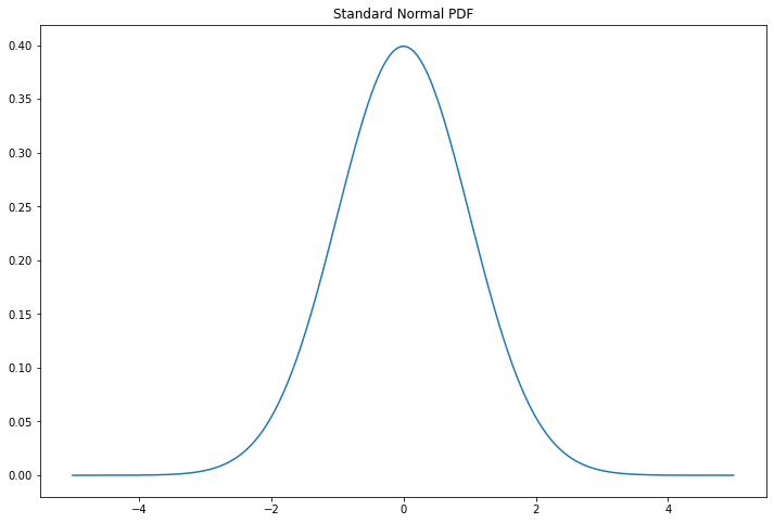
png
There is no closed-form expression for \(\Phi\). Here are some useful facts:
If \(X \sim N(\mu, \sigma^2)\) then \(Z = (X - \mu) / \sigma \sim N(0, 1)\)
If \(Z \sim N(0, 1)\) then \(X = \mu + \sigma Z \sim N(\mu, \sigma^2)\)
If \(X_i \sim N(\mu_i, \sigma_i^2)\), \(i = 1, \dots, n\) are independent then
\[ \sum_{i=1}^n X_i \sim N \left(\sum_{i=1}^n \mu_u, \sum_{i=1}^n \sigma_i^2 \right) \]
It follows from the first fact that if \(X \sim N(\mu, \sigma^2)\) then
\[ \mathbb{P}(a < X < b) = \mathbb{P}\left( \frac{a - \mu}{\sigma} < Z < \frac{b - \mu}{\sigma} \right) = \Phi \left( \frac{b - \mu}{\sigma} \right) - \Phi \left( \frac{a - \mu}{\sigma} \right) \]
Thus we can compute any probabilities we want as long as we can compute the CDF \(\Phi(z)\) of the standard Normal. All statistical and computing packages will compute \(\Phi(z)\) and \(\Phi^{-1}(q)\).
Exponential Distribution
\(X\) has an exponential distribution with parameter \(\beta\), denoted by \(X \sim \text{Exp}(\beta)\), if
\[ f(x) = \frac{1}{\beta} e^{-x / \beta}, \quad x > 0 \]
where \(\beta > 0\). The exponential distribution is used to model the lifetimes of electronic components and the waiting times between rare events.
Gamma Distribution
For \(\alpha > 0\), the Gamma function is defined by \(\Gamma(\alpha) = \int_0^\infty y^{\alpha - 1} e^{-y} dy\). \(X\) has a Gamma distribution with parameters \(\alpha\) and \(\beta\), denoted by \(X \sim \text{Gamma}(\alpha, \beta)\), if
\[ f(x) = \frac{1}{\beta^\alpha \Gamma(\alpha)} x^{\alpha - 1} e^{-x / \beta}, \quad x > 0 \]
where \(\alpha, \beta > 0\). The exponential distribution is just a \(\text{Gamma}(1, \beta)\) distribution. If \(X_i \sim \text{Gamma}(\alpha_i, \beta)\) are independent, then \(\sum_{i=1}^n X_i \sim \text{Gamma}\left( \sum_{i=1}^n \alpha_i, \beta \right)\).
Beta Distribution
\(X\) has Beta distribution with parameters \(\alpha > 0\) and \(\beta > 0\), denoted by \(X \sim \text{Beta}(\alpha, \beta)\), if
\[ f(x) = \frac{\Gamma(\alpha + \beta)}{\Gamma(\alpha) \Gamma(\beta)} x^{\alpha - 1} (1 - x)^{\beta - 1}, \quad 0 < x < 1\]
\(t\) and Cauchy Distribution
\(X\) has a \(t\) distribution with \(\nu\) degrees of freedom – written \(X \sim t_\nu\) – if
\[ f(x) = \frac{1}{\sqrt{\nu \pi}} \frac{\Gamma\left( \frac{\nu + 1}{2} \right)}{\Gamma\left( \frac{\nu}{2} \right)} \frac{1}{\left(1 + \frac{x^2}{\nu} \right)^{(\nu + 1) / 2}} \]
The \(t\) distribution is similar to a Normal but it has thicker tails. In fact, the Normal corresponds to a \(t\) with \(\nu = \infty\). The Cauchy distribution is a special case of the \(t\) distribution corresponding to \(\nu = 1\). The density is
\[ f(x) = \frac{1}{\pi (1 + x^2)} \]
The \(\chi^2\) Distribution
\(X\) has a \(\chi^2\) distribution with \(p\) degrees of freedom – written \(X \sim \chi_p^2\) – if
\[ f(x) = \frac{1}{\Gamma\left(\frac{p}{2}\right) 2^{\frac{p}{2}}} x^{\frac{p}{2} - 1} e^{-\frac{x}{2}}, \quad x > 0 \]
If \(Z_1, Z_2, \dots\) are independent standard Normal random variables then \(\sum_{i=1}^p Z_i^2 \sim \chi_p^2\).
3.5 Bivariate Distributions
Given a pair of discrete random variables \(X\) and \(Y\), define the joint mass function by \(f(x, y) = \mathbb{P}(X = x \text{ and } Y = y)\). From now on, we write \(\mathbb{P}(X = x \text{ and } Y = y)\) as \(\mathbb{P}(X = x, Y = y)\). We write \(f\) as \(f_{X, Y}\) when we want to be more explicit.
In the continuous case, we call a function \(f(x, y)\) a PDF for the random variables \((X, Y)\) if:
- \(f(x, y) \geq 0\) for all \((x, y)\)
- \(\int_{-\infty}^\infty \int_{-\infty}^\infty f(x, y) \; dx dy = 1\)
- For any set \(A \subset \mathbb{R} \times \mathbb{R}\), \(\mathbb{P}((X, Y) \in A) = \int \int_A f(x, y) \; dx dy\)
In the continuous or discrete case, we define the joint CDF as $ F_{X, Y}(x, y) = (X x, Y y) $.
3.6 Marginal Distributions
If \((X, Y)\) have joint distribution with mass function \(f_{X, Y}\), then the marginal mass function for \(X\) is defined by
\[ f_X(x) = \mathbb{P}(X = x) = \sum_y \mathbb{P}(X = x, Y = y) = \sum_y f(x, y) \]
and the marginal mass function for \(Y\) is defined by
\[ f_Y(y) = \mathbb{P}(Y = y) = \sum_x \mathbb{P}(X = x, Y = y) = \sum_x f(x, y) \]
For continuous random variables, the marginal densities are
\[ f_X(x) = \int f(x, y) \; dy \quad \text{and} \quad f_Y(y) = \int f(x, y) \; dx \]
The corresponding marginal CDFs are denoted by \(F_X\) and \(F_Y\).
3.7 Independent Random Variables
Two random variables \(X\) and \(Y\) are independent if, for every \(A\) and \(B\),
\[ \mathbb{P}(X \in A, Y \in B) = \mathbb{P}(X \in A) \mathbb{P}(Y \in B) \]
We write \(X \text{ ⫫ } Y\).
In principle, to check whether \(X\) and \(Y\) are independent we need to check the equation above for all subsets \(A\) and \(B\). Fortunately, we have the following result which we state for continuous random variables though it is true for discrete random variables too.
Theorem 3.30. Let \(X\) and \(Y\) have joint PDF \(f_{X, Y}\). Then \(X \text{ ⫫ } Y\) if and only if \(f_{X, Y}(x, y) = f_X(x) f_Y(y)\) for all values \(x\) and \(y\).
The statement is not rigorous because the density is defined only up to sets of measure 0.
The following result is helpful for verifying independence.
Theorem 3.33. Suppose that the range of \(X\) and \(Y\) is a (possibly infinite) rectangle. If \(f(x, y) = g(x) h(y)\) for some functions \(g\) and \(h\) (not necessarily probability density functions) then \(X\) and \(Y\) are independent.
3.8 Conditional Distributions
The conditional probability mass function is
\[ f_{X | Y}(x | y) = \mathbb{P}(X = x | Y = y) = \frac{\mathbb{P}(X = x, Y = y)}{\mathbb{P}(Y = y)} = \frac{f_{X, Y}(x, y)}{f_Y(y)} \]
if \(f_Y(y) > 0\).
For continuous random variables, the conditional probability density function is
\[ f_{X | Y}(x | y) = \frac{f_{X, Y}(x, y)}{f_Y(y)} \]
assuming that \(f_Y(y) > 0\). Then,
\[ \mathbb{P}(X \in A | Y = y) = \int_A f_{X | Y}(x | y) \; dx \]
We are treading in deep water here. When we compute \(\mathbb{P}(X \in A | Y = y)\) in the continuous case we are conditioning on the event \(\mathbb{P}(Y = y)\) which has probability 0. We avoid this problem by defining things in terms of the PDF. The fact that this leads to a well-defined theory is proved in more advanced courses. We simply take it as a definition.
3.9 Multivariate Distributions and IID Samples
Let \(X = (X_1, \dots, X_n)\) where the \(X_i\)’s are random variables. We call \(X\) a random vector. Let \(f(x_1, \dots, x_n)\) denote the PDF. It is possible to define their marginals, conditionals, etc. much the same way as in the bivariate case. We say that \(X_1, \dots, X_n\) are independent if, for every \(A_1, \dots, A_n\),
\[ \mathbb{P}(X_1 \in A_1, \dots, X_n \in A_n) = \prod_{i=1}^n \mathbb{P}(X_i \in A_i) \]
It suffices to check that \(f(x_1, \dots, x_n) = \prod_{i=1}^n f_{X_i}(x_i)\). If \(X_1, \dots, X_n\) are independent and each has the same marginal distribution with density \(f\), we say that \(X_1, \dots, X_n\) are IID (independent and identically distributed). We shall write this as \(X_1, \dots, X_n \sim f\) or, in terms of the CDF, \(X_1, \dots, X_n \sim F\). This means that \(X_1, \dots, X_n\) are independent draws from the same distribution. We also call \(X_1, \dots, X_n\) a random sample from \(F\).
3.10 Two Important Multivariate Distributions
Multinomial Distribution
The multivariate version of the Binomial is called a Multinomial. Consider drawing a ball from an urn which has balls of \(k\) different colors. Let \(p = (p_1, \dots, p_k)\) where \(p_j \geq 0\) and \(\sum_{j=1}^k p_j = 1\) and suppose that \(p_j\) is the probability of drawing a ball of color \(j\). Draw \(n\) times (independent draws with replacement) and let \(X = (X_1, \dots, X_k)\), where \(X_j\) is the number of times that color \(j\) appears. Hence, \(n = \sum_{j=1}^k X_j\). We say that \(X\) has a Multinomial distribution with parameters \(n\) and \(p\), written \(X \sim \text{Multinomial}(n, p)\). The probability function is
\[ f(x) = \binom{n}{x_1 \cdots x_k} p_1^{x_1} \cdots p_k^{x_k} \]
where
\[ \binom{n}{x_1 \cdots x_k} = \frac{n!}{x_1! \cdots x_k!} \]
Lemma 3.41. Suppose that \(X \sim \text{Multinomial}(n, p)\) where \(X = (X_1, \dots, X_k)\) and \(p = (p_1, \dots, p_k)\). The marginal distribution of \(X_j\) is \(\text{Binomial}(n, p_j)\).
Multivariate Normal
The univariate Normal had two parameters, \(\mu\) and \(\sigma\). In the multivariate vector, \(\mu\) is a vector and \(\sigma\) is replaced by a matrix \(\Sigma\). To begin, let
\[ Z = \begin{pmatrix} Z_1 \\ \vdots \\ Z_k \end{pmatrix}\]
where \(Z_1, \dots, Z_k \sim N(0, 1)\) are independent. The density of \(Z\) is
\[ f(z) = \prod_{i=1}^k f(z_i) = \frac{1}{(2 \pi)^{k/2}} \exp \left\{ -\frac{1}{2} \sum_{j=1}^k z_j^2 \right\} = \frac{1}{(2 \pi)^{k/2}} \exp \left\{ -\frac{1}{2} z^T z \right\} \]
We say that \(Z\) has a standard multivariate Normal distribution, written \(Z \sim N(0, I)\) where it is understood that \(0\) represents a vector of \(k\) zeroes and \(I\) is the \(k \times k\) identity matrix.
More generally, a vector \(X\) has multivariate Normal distribution, denoted by \(X \sim N(\mu, \Sigma)\), if it has density
\[ f(x; \mu, \Sigma) = \frac{1}{(2 \pi)^{k/2} \text{det}(\Sigma)^{1/2}} \exp \left\{ - \frac{1}{2} (x - \mu)^T \Sigma^{-1} (x - \mu) \right\} \]
where \(\text{det}(\cdot)\) denotes the determinant of a matrix, \(\mu\) is a vector of length \(k\), and \(\Sigma\) is a \(k \times k\) symmetric, positive definite matrix. Setting \(\mu = 0\) and \(\Sigma = I\) gives back the standard Normal.
A matrix \(\Sigma\) is positive definite if, for all non-zero vectors \(x\), \(x^T \Sigma x > 0\).
Since \(\Sigma\) is symmetric and positive definite, it can be shown that there exists a matrix \(\Sigma^{1/2}\) – called the square root of \(\Sigma\) – with the following properties:
- \(\Sigma^{1/2}\) is symmetric
- \(\Sigma = \Sigma^{1/2} \Sigma^{1/2}\)
- \(\Sigma^{1/2}\Sigma^{-1/2} = \Sigma^{-1/2}\Sigma^{1/2} = I\), where \(\Sigma^{1/2} = \left(\Sigma^{1/2}\right)^{-1}\)
Theorem 3.42. If \(Z \sim N(0, I)\) and \(X = \mu + \Sigma^{1/2} Z\) then \(X \sim N(\mu, \Sigma)\). Conversely, if \(X \sim N(\mu, \Sigma)\), then \(\Sigma^{-1/2}(X - \mu) \sim N(0, I)\).
Suppose we partition a random Normal vector \(X\) as \(X = (X_a, X_b)\), and we similarly partition
\[ \mu = \begin{pmatrix}\mu_a & \mu_b \end{pmatrix} \quad \Sigma = \begin{pmatrix} \Sigma_{aa} & \Sigma_{ab} \\ \Sigma_{ba} & \Sigma_{bb} \end{pmatrix} \]
Theorem 3.43. Let \(X \sim N(\mu, \Sigma)\). Then:
The marginal distribution of \(X_a\) is \(X_a \sim N(\mu_a, \Sigma_{aa})\).
The conditional distribution of \(X_b\) given \(X_a = x_a\) is
\[ X_b | X_a = x_a \sim N \left( \mu_b + \Sigma_{ba}\Sigma_{aa}^{-1}(x_a - \mu_a), \Sigma_{bb} - \Sigma_{ba} \Sigma_{aa}^{-1} \Sigma_{ab} \right) \]
If \(a\) is a vector then \(a^T X \sim N(a^T \mu, a^T \Sigma a)\)
\(V = (X - \mu)^T \Sigma^{-1} (X - \mu) \sim \chi_k^2\)
3.11 Transformations of Random Variables
Suppose that \(X\) is a random variable with PDF \(f_X\) and CDF \(F_X\). Let \(Y = r(X)\) be a function of \(X\), such as \(Y = X^2\) or \(Y = e^X\). We call \(Y = r(X)\) a transformation of \(X\). How do we compute the PDF and the CDF of \(Y\)? In the discrete case, the answer is easy. The mass function of \(Y\) is given by
\[ f_Y(y) = \mathbb{P}(Y = y) = \mathbb{P}(r(X) = y) = \mathbb{P}(\{x; r(x) = y\}) = \mathbb{P}(X \in r^{-1}(y)) \]
The continuous case is harder. There are 3 steps for finding \(f_Y\):
For each \(y\), find the set \(A_y = \{ x : r(x) \leq y \}\).
Find the CDF
\[ F_Y(y) = \mathbb{P}(Y \leq y) = \mathbb{P}(r(X) \leq y) = \mathbb{P}(\{x ; r(x) \leq y \}) = \int_{A_y} f_X(x) dx \]
The PDF is \(f_Y(y) = F'_Y(y)\).
When \(r\) is strictly monotone increasing or strictly monotone decreasing then \(r\) has an inverse \(s = r^{-1}\) and in this case one can show that
\[ f_Y(y) = f_X(s(y)) \;\Bigg| \frac{ds(y)}{dy} \Bigg|\]
3.12 Transformation of Several Random Variables
In some cases we are interested in the transformation of several random variables. For example, if \(X\) and \(Y\) are given random variables, we might want to know the distribution of \(X / Y\), \(X + Y\), \(\max \{ X, Y \}\) or \(\min \{ X, Y \}\). Let \(Z = r(X, Y)\). The steps for finding \(f_Z\) are the same as before:
- For each \(z\), find the set \(A_z = \{ (x, y) : r(x, y) \leq z \}\).
- Find the CDF
\[ F_Z(z) = \mathbb{P}(Z \leq z) = \mathbb{P}(r(X, Y) \leq z) = \mathbb{P}(\{ (x, y) : r(x, y) \leq z \}) = \int \int_{A_z} f_{X, Y}(x, y) \; dx dy \]
- Find \(f_Z(z) = F'_Z(z)\).
3.13 Technical Appendix
Recall that a probability measure \(\mathbb{P}\) is defined on a \(\sigma\)-field \(\mathcal{A}\) of a sample space \(\Omega\). A random variable \(X\) is measurable map \(X : \Omega \rightarrow \mathbb{R}\). Measurable means that, for every \(x\), ${ : X() x } $.
3.14 Exercises
Exercise 3.14.1. Show that
\[ \mathbb{P}(X = x) = F(x^+) - F(x^-) \]
and
\[ F(x_2) - F(x_1) = \mathbb{P}(X \leq x_2) - \mathbb{P}(X \leq x_1) \]
Solution.
By definition, \(F(x_2) = \mathbb{P}(X \leq x_2)\) and \(F(x_1) = \mathbb{P}(X \leq x_1)\), so the second equation is immediate.
Also by definition,
\[ F(x^+) = \lim_{y \rightarrow x, y > x} F(y) = \lim_{y \rightarrow x, y > x} \mathbb{P}(X \leq y) = \mathbb{P}(\exists y : X \leq y, y > x) = \mathbb{P}(X \leq x) \]
and
\[ F(x^-) = \lim_{y \rightarrow x, y < x} F(y) = \lim_{y \rightarrow x, y > x} \mathbb{P}(X \leq y) = \mathbb{P}(\exists y : X \leq y, y < x) = \mathbb{P}(X < x) \]
and so
\[ F(x^+) - F(x^-) = \mathbb{P}(X \leq x) - \mathbb{P}(X < x) = \mathbb{P}(X(\omega) \in \{x : X(\omega) \leq x \} - \{x: X(\omega) < x \}) = \mathbb{P}(X = x)\]
Exercise 3.14.2. Let \(X\) be such that \(\mathbb{P}(X = 2) = \mathbb{P}(X = 3) = 1/10\) and \(\mathbb{P}(X = 5) = 8/10\). Plot the CDF \(F\). Use \(F\) to find \(\mathbb{P}(2 < X \leq 4.8)\) and \(\mathbb{P}(2 \leq X \leq 4.8)\).
Solution.
import numpy as np
import matplotlib.pyplot as plt
%matplotlib inline

plt.figure(figsize=(12, 8))

# Draw horizontal lines
for xmin, xmax, y in [(0, 2, 0), (2, 3, 1/10), (3, 5, 2/10), (5, 10, 1)]:
    plt.hlines(y, xmin, xmax, color='C0', linestyle='solid')

# Draw vertical lines
for ymin, ymax, x in [(0, 1/10, 2), (1/10, 2/10, 3), (2/10, 1, 5)]:
    plt.vlines(x, ymin, ymax, color='C0', linestyle='dashed')

# Mark open intervals
plt.scatter([2, 3, 5], [0, 1/10, 2/10], color='C0', facecolor='white', zorder=10, linewidth=2)

# Mark close intervals
plt.scatter([2, 3, 5], [1/10, 2/10, 1], color='C0', facecolor='C0', zorder=10, linewidth=2)

plt.xlabel('x')
plt.ylabel('F(x)')
plt.show()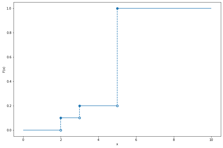
png
\[ \mathbb{P}(2 < X \leq 4.8) = F(4.8) - F(2) = 0.2 - 0.1 = 0.1 \quad \text{ and } \quad \mathbb{P}(2 \leq X \leq 4.8) = F(4.8) - F(2^{-}) = 0.2 - 0 = 0.2 \]
Exercise 3.14.3. Prove Lemma 3.15.
Let \(F\) be the CDF for a random variable \(X\). Then:
\(\mathbb{P}(X = x) = F(x) - F(x^-)\) where \(F(x^-) = \lim_{y \to x} F(y)\)
\(\mathbb{P}(x < X \leq y) = F(y) - F(x)\)
\(\mathbb{P}(X > x) = 1 - F(x)\)
If \(X\) is continuous then
\[ \mathbb{P}(a < X < b) = \mathbb{P}(a \leq X < b) = \mathbb{P}(a < X \leq b) = \mathbb{P}(a \leq X \leq b) \]
Solution.
Proof of first statement:
\[ F(x) - F(x^{-}) = \mathbb{P}(X \leq x) - \mathbb{P}(X < x) = \mathbb{P}(\{\omega : X(\omega) \leq x\} - \{\omega : X(\omega) < x\}) = \mathbb{P}(X = x)\]
Proof of second statement:
\[ \mathbb{P}(x < X \leq y) = \mathbb{P}(\{\omega : X(\omega) \leq y\} - \{\omega : X(\omega) \leq x\}) = \mathbb{P}(X \leq y) - \mathbb{P}(X \leq x) = F(y) - F(x) \]
Proof of third statement:
\[ \mathbb{P}(X > x) = \mathbb{P}(\{\omega: X(\omega) > x\}) = \mathbb{P}(\{\omega: X(\omega) \leq x\}^c) = 1 - \mathbb{P}(X \leq x) = 1 - F(x) \]
Proof of fourth statement:
If \(F\) is continuous, then \(\mathbb{P}(X = a) = \mathbb{P}(X = b) = 0\), and so
\[ \begin{align} \mathbb{P}(a < X \leq b) &= \mathbb{P}(a < X < b) + \mathbb{P}(X = b) = \mathbb{P}(a < X < b) \\ \mathbb{P}(a \leq X < b) &= \mathbb{P}(X = a) + \mathbb{P}(a < X < b) = \mathbb{P}(a < X < b) \\ \mathbb{P}(a \leq X \leq b) &= \mathbb{P}(X = a) + \mathbb{P}(a < X < b) + \mathbb{P}(X = b) = \mathbb{P}(a < X < b) \end{align} \]
Exercise 3.14.4. Let \(X\) have probability density function
\[ f_X(x) = \begin{cases} 1/4 &\text{if } 0 < x < 1 \\ 3/8 &\text{if } 3 < x < 5 \\ 0 &\text{otherwise} \end{cases} \]
(a) Find the cumulative distribution function of \(X\).
(b) Let \(Y = 1 / X\). Find the probability density function \(f_Y(y)\) for \(Y\). Hint: Consider three cases, \(\frac{1}{5} \leq y \leq \frac{1}{3}\), \(\frac{1}{3} \leq y \leq 1\), and \(y \geq 1\).
Solution.
(a)
\[ F_X(x) = \begin{cases} 0 &\text{if } x \leq 0 \\ \frac{x}{4} &\text{if } 0 < x < 1 \\ \frac{1}{4} &\text{if } 1 \leq x < 3 \\ \frac{1}{4} + \frac{3(x - 3)}{8} &\text{if } 3 \leq x < 5 \\ 1 &\text{if } x \geq 5 \end{cases} \]
import numpy as np
import matplotlib.pyplot as plt
%matplotlib inline

plt.figure(figsize=(12, 8))

# Draw horizontal lines
for xmin, xmax, y in [(-2, 0, 0), (1, 3, 1/4), (5, 7, 1)]:
    plt.hlines(y, xmin, xmax, color='C0', linestyle='solid')

# Draw diagonal lines
for x1, y1, x2, y2 in [(0, 0, 1, 1/4), (3, 1/4, 5, 1)]:
    plt.plot([x1, x2], [y1, y2], color='C0')

plt.xlabel(r'$x$')
plt.ylabel(r'$F(x)$')
plt.show()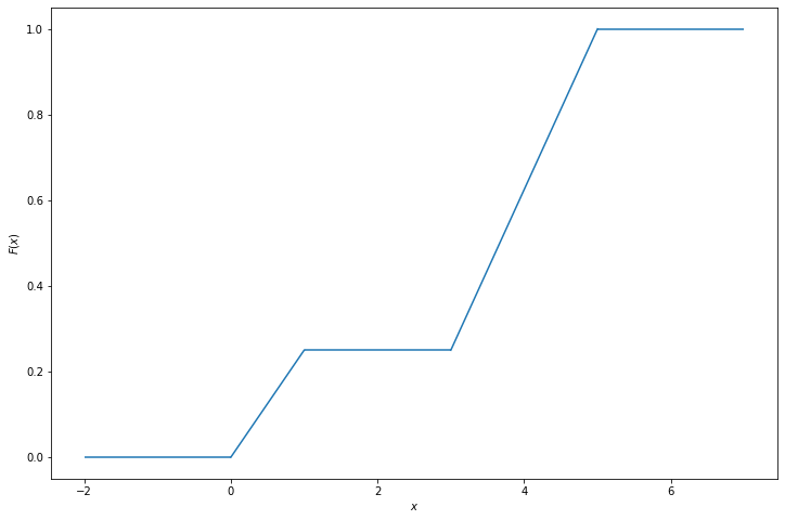
png
(b)
\(\mathbb{P}(X > 0) = 1\), so \(\mathbb{P}(Y > 0) = 1\). For \(y > 0\), we have:
\[ F_Y(y) = \mathbb{P}(Y \leq y) = \mathbb{P}\left(\frac{1}{X} \leq y\right) = \mathbb{P}\left(X \geq \frac{1}{y}\right) = 1 - F_X\left(\frac{1}{y} \right) \]
so
\[ F_Y(y) = \begin{cases} 0 &\text{if } y \leq \frac{1}{5} \\ \frac{15}{8} - \frac{3}{8y} &\text{if } \frac{1}{5} < y \leq \frac{1}{3} \\ \frac{3}{4} &\text{if } \frac{1}{3} < y \leq 1 \\ 1 - \frac{1}{4y} &\text{if } y > 1 \end{cases} \]
import numpy as np
import matplotlib.pyplot as plt
%matplotlib inline

plt.figure(figsize=(12, 8))

# Draw horizontal lines
for xmin, xmax, y in [(-2, 1/5, 0), (1/3, 1, 3/4)]:
    plt.hlines(y, xmin, xmax, color='C0')


# Draw increasing segments
yy = np.arange(1/5, 1/3, step=0.001)
plt.plot(yy, 15/8 - 3/(8 * yy), color='C0')

yy = np.arange(1, 8, step=0.01)
plt.plot(yy, 1 - 1/(4*yy), color='C0')

plt.xlabel(r'$y$')
plt.ylabel(r'$F_Y(y)$')
plt.show()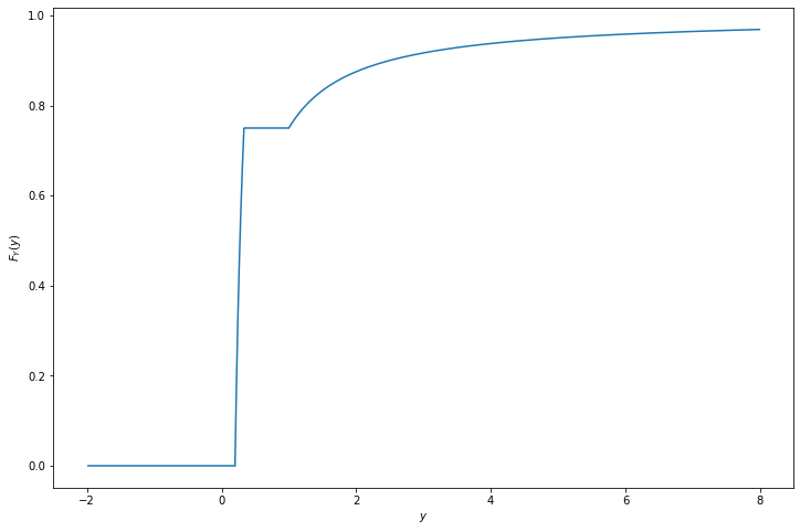
png
The probability density function is \(f_y(y) = F'_Y(y)\), so
\[ f_Y(y) = \begin{cases} 0 &\text{if } y \leq \frac{1}{5} \\ \frac{3}{8y^2} &\text{if } \frac{1}{5} < y \leq \frac{1}{3} \\ 0 &\text{if } \frac{1}{3} < y \leq 1 \\ \frac{1}{4y^2} &\text{if } y > 1 \end{cases}\]
import numpy as np
import matplotlib.pyplot as plt
%matplotlib inline

def f_Y(y):
    return np.where(y <= 1/5, 0, np.where(y <= 1/3, 3/(8 * (y**2)), np.where(y <= 1, 0, 1/(4 * (y**2)))))

plt.figure(figsize=(12, 8))

yy = np.arange(-1, 3, step=0.001)
plt.plot(yy, f_Y(yy), color='C0')

plt.xlabel(r'$y$')
plt.ylabel(r'$f_Y(y)$')
plt.show()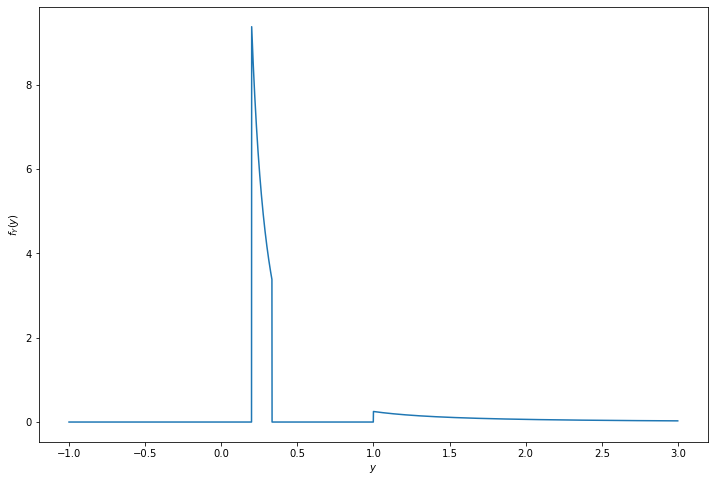
png
Exercise 3.14.5. Let \(X\) and \(Y\) be discrete random variables. Show that \(X\) and \(Y\) are independent if and only if \(f_{X, Y}(x, y) = f_X(x) f_Y(y)\) for all \(x\) and \(y\).
Solution. If \(x\) or \(y\) take values that have probability mass 0, then trivially \(f_{X, Y}(x, y) = 0\) and \(f_X(x) f_Y(y) = 0\), so we only need to consider \(x\) and \(y\) with positive probability mass.
If \(X\) and \(Y\) are independent, then \(\mathbb{P}(X \in A, Y \in B) = \mathbb{P}(X \in A)\mathbb{P}(Y \in B)\) for all events \(A\), \(B\). In particular, this is true for \(A = \{x\}\) and \(B = \{ y \}\) for all \(x, y\), proving the implication in one direction.
In the other direction, we have
\[ \mathbb{P}(X \in A, Y \in B) = \sum_{x \in A} \sum_{y \in B} f_{X, Y}(x, y) \]
and
\[ \mathbb{P}(X \in A) = \sum_{x \in A} f_X(x) \quad \text{and} \quad \mathbb{P}(Y \in B) = \sum_{y \in B} f_Y(y) \]
so \(f_{X, Y}(x, y) = f_X(x) f_Y(y)\) for all \(x, y\) implies that for all \(A\) and \(B\),
\[ \mathbb{P}(X \in A) \mathbb{P}(Y \in B) = \left( \sum_{x \in A} f_X(x) \right) \left( \sum_{y \in B} f_Y(y) \right) = \sum_{x \in A} \sum_{y \in B} f_X(x) f_Y(y) = \sum_{x \in A} \sum_{y \in B} f_{X, Y}(x, y) = \mathbb{P}(X \in A, Y \in B) \]
so \(X, Y\) are independent, proving the implication in the other direction.
Exercise 3.14.6. Let \(X\) have distribution \(F\) and density function \(f\) and let \(A\) be a subset of the real line. Let \(I_A(x)\) be the indicator function for \(A\):
\[ I_A(x) = \begin{cases} 1 &\text{if } x \in A \\ 0 &\text{otherwise} \end{cases} \]
Let \(Y = I_A(X)\). Find an expression for the cumulative distribution function of \(Y\). (Hint: first find the mass function for \(Y\).)
Solution. Note that \(I_A\) can only return values 0 or 1, so \(Y\) is a discrete variable with non-zero probability mass only at values 0 and 1.
But $(Y = 1) = (x A) = _A f_X(x) dx $, so the PDF for \(Y\) is:
\[ f_Y(y) = \begin{cases} \int_A f_X(x) dx &\text{if } y = 1 \\ 1 - \int_A f_X(x) dx &\text{if } y = 0 \\ 0 &\text{otherwise} \end{cases} \]
and so the CDF of \(Y\) is:
\[ F_Y(y) = \begin{cases} 0 &\text{if } y < 0 \\ 1 - \int_A f_X(x) dx &\text{if } 0 \leq y < 1 \\ 1 &\text{if } y \geq 1 \end{cases} \]
Exercise 3.14.7. Let \(X\) and \(Y\) be independent and suppose that each has a \(\text{Uniform}(0, 1)\) distribution. Let \(Z = \min \{ X, Y \}\). Find the density \(f_Z(z)\) for \(Z\). Hint: it might be easier to first find \(\mathbb{P}(Z > z)\).
Solution.
\[1 - F_Z(z) = \mathbb{P}(Z > z) = \mathbb{P}(X > z, Y > z) = (1 - F_X(z)) (1 - F_Y(z)) \]
But \(F_X\) and \(F_Y\) are both the CDF of the \(\text{Uniform}(0, 1)\) distribution, so
\[ F_X(x) = \begin{cases} 0 &\text{if } x \leq 0 \\ x &\text{if } 0 < x \leq 1 \\ 1 &\text{if } x > 1 \end{cases} \]
and so
\[ F_Z(z) = \begin{cases} 0 &\text{if } z \leq 0 \\ 2z - z^2 &\text{if } 0 < z \leq 1 \\ 1 &\text{if } z > 1 \end{cases} \]
and the PDF is \(f_Z(z) = F'_Z(z)\):
\[ f_Z(z) = \begin{cases} 0 &\text{if } z \leq 0 \\ 2 - 2z &\text{if } 0 < z < 1 \\ 0 &\text{if } z > 1 \end{cases} \]
import numpy as np
import matplotlib.pyplot as plt
%matplotlib inline

def f_Z(z):
    return np.where(z <= 0, 0, np.where(z >= 1, 0, 2 - 2 * z))

plt.figure(figsize=(12, 8))

zz = np.arange(-0.5, 1.5, step=0.01)
plt.plot(zz, f_Z(zz), color='C0')

plt.xlabel(r'$z$')
plt.ylabel(r'$f_Z(z)$')
plt.show()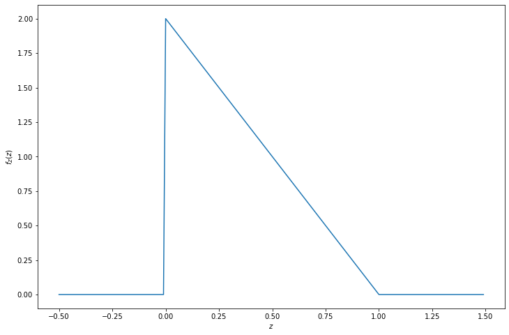
png
Exercise 3.14.8. Let \(X\) have CDF \(F\). Find the CDF of \(X^+ = \max \{0, X\}\).
Solution.
\[ F_{X^+}(x) = \mathbb{P}(X^+ \leq x) = \mathbb{P}(0 < x, X < x) = I(0 < x) F_X(x) \]
Exercise 3.14.9. Let \(X \sim \text{Exp}(\beta)\). Find \(F(x)\) and \(F^{-1}(q)\).
Solution. Let’s start from the definition for the PDF of the exponential distribution:
\[ f(x) = \frac{1}{\beta} e^{-x / \beta}, \quad x > 0 \]
We have:
\[ F(x) = \int_{0}^x f(t) dt = \int_{0}^x \frac{1}{\beta} e^{-t / \beta} dt = \frac{1}{\beta} \beta \left( 1 - e^{-x / \beta} \right) = 1 - e^{-x / \beta} \]
and so
\[ q = 1 - e^{-F^{-1}(q) / \beta} \Longrightarrow F^{-1}(q) = -\beta \log (1 - q) \]
Exercise 3.14.10. Let \(X\) and \(Y\) be independent. Show that \(g(X)\) is independent of \(h(Y)\) where \(g\) and \(h\) are functions.
Solution. Let \(g^{-1}(A) = \{ x : g(x) \in A \}\) and \(h^{-1}(B) = \{ y : h(y) \in B \}\). We have:
\[\mathbb{P}(g(X) \in A, h(Y) \in B) = \mathbb{P}(X \in g^{-1}(A), Y \in h^{-1}(B)) = \mathbb{P}(X \in g^{-1}(A)) \mathbb{P}(Y \in h^{-1}(B)) = \mathbb{P}(g(X) \in A) \mathbb{P}(h(Y) \in B)\]
Exercise 34.14.11. Suppose we toss a coin once and let \(p\) be the probability of heads. Let \(X\) denote the number of heads and \(Y\) denote the number of tails.
(a) Prove that \(X\) and \(Y\) are dependent.
(b) Let \(N \sim \text{Poisson}(\lambda)\) and suppose that we toss a coin \(N\) times. Let \(X\) and \(Y\) be the number of heads and tails. Show that \(X\) and \(Y\) are independent.
Solution.
(a) The joint probability mass function is:
\[ \begin{array}{c|cc} f_{X, Y} & Y = 0 & Y = 1 \\ \hline X = 0 & 0 & 1 - p\\ X = 1 & p & 0 \end{array} \]
In particular, \(f_{X, Y}(1, 0) = p\) and \(f_X(1) f_Y(0) = p^2\), so the events are dependent unless \(p \in \{0, 1\}\).
(b) The joint probability mass function is:
\[ \mathbb{P}(X = x, Y = y) = \mathbb{P}(N = x + y, X = x) = \frac{\lambda^{x+y}e^{-\lambda}}{(x + y)!} \binom{x + y}{x} p^x (1-p)^y = e^{-\lambda} \left(\frac{\lambda^x}{x!} p^x \right) \left(\frac{\lambda^y}{y!} (1 - p)^y\right) = g(x) h(y)\]
where \(g(x)=e^{-\lambda}\frac{\lambda^x}{x!}p^x\), \(h(y) = \frac{\lambda^y}{y!} (1 - p)^y\). The result then follows from theorem 3.33.
Exercise 3.14.12. Prove theorem 3.33.
Suppose that the range of \(X\) and \(Y\) is a (possibly infinite) rectangle. If \(f(x, y) = g(x) h(y)\) for some functions \(g\) and \(h\) (not necessarily probability density functions) then \(X\) and \(Y\) are independent.
Solution.
Given that \(F\) is the joint probability density function of \(X\) and \(Y\), then the marginal distributions for \(X\) and \(Y\) are
\[ f_X(x) = \int f(x, y) dy = \int g(x) h(y) dy = g(x) \int h(y) dy = H g(x) \quad \text{ for some constant } H \]
and
\[ f_Y(y) = \int f(x, y) dx = \int g(x) h(y) dx = h(y) \int g(x) dx = G h(y) \quad \text{ for some constant } G \]
Therefore,
\[ f_X(x) f_Y(y) = HG g(x) h(y) = HG f(x, y) \]
Integrating over \(x\), and fixing \(y = y_0\) with non-zero probability density,
\[ \int f_X(x) f_Y(y_0) dx = HG \int f(x, y_0) dx \Longrightarrow f_Y(y_0) = HG f_Y(y_0) \Longrightarrow HG = 1 \]
and so
\[ f_X(x) f_Y(y) = f(x, y) \]
therefore \(X\) and \(Y\) are independent.
Exercise 3.14.13. Let \(X \sim N(0, 1)\) and let \(Y = e^X\).
(a) Find the PDF for \(Y\). Plot it.
(b) (Computer Experiment) Generate a vector \(x = (x_1, \dots, x_{10,000})\) consisting of 10,000 random standard Normals. Let \(y = (y_1, \dots, y_{10,000})\) where \(y_i = e^{x_i}\). Draw a histogram of \(y\) and compare it to the PDF you found in part (a).
Solution.
(a)
Assuming \(y > 0\),
\[ F_Y(y) = \mathbb{P}(Y \leq y) = \mathbb{P}(X \leq \log y) = \Phi(\log y) \]
and so
\[ f_Y(y) = \frac{d}{dy} \Phi(\log y) = \frac{d \Phi(\log y)}{d \log y} \frac{d \log y}{dy} = \frac{\phi(\log(y))}{y} \]
And, of course, \(Y\) can never take a negative value, so
\[ f_Y(y) = \begin{cases} \frac{\phi(\log(y))}{y} &\text{if } y > 0 \\ 0 &\text{otherwise} \end{cases} \]
import numpy as np
from scipy.stats import norm

import matplotlib.pyplot as plt
%matplotlib inline

yy = np.arange(0.01, 5, step=0.01)

def f_Y(y):
    return norm.pdf(np.log(y)) / y

plt.figure(figsize=(12, 8))
plt.plot(yy, f_Y(yy))
plt.xlabel(r'$y$')
plt.ylabel(r'$f_Y(y)$')
plt.show()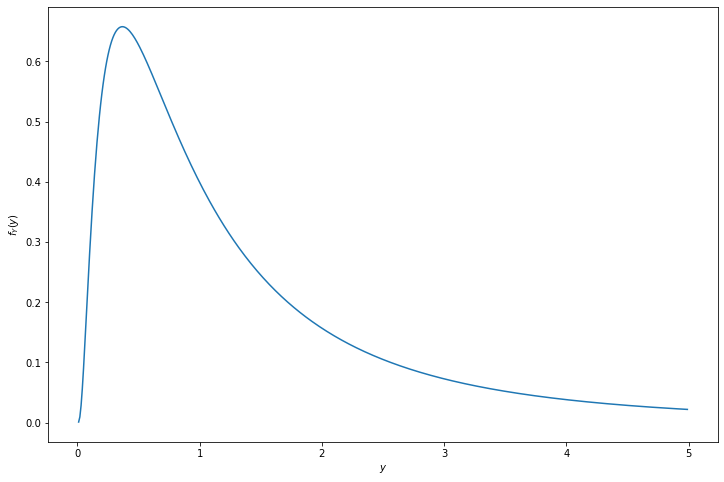
png
(b)
np.random.seed(0)

N = 10000
X = norm.rvs(size=N)
Y = np.exp(X)

plt.figure(figsize=(12, 8))
plt.hist(Y, bins=200, density=True, label='histogram', histtype='step')
plt.plot(yy, f_Y(yy), label='true density')
plt.legend(loc='upper right')
plt.xlim(0, 5)
plt.show()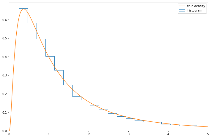
png
Exercise 3.14.14. Let \((X, Y)\) be uniformly distributed on the unit disc \(\{ (x, y) : x^2 + y^2 \leq 1 \}\). Let \(R = \sqrt{X^2 + Y^2}\). Find the CDF and the PDF of \(R\).
Solution.
Assuming \(r > 0\),
\[ F_R(r) = \mathbb{P}(R \leq r) = \mathbb{P}(X^2 + Y^2 \leq r^2) = \int \int_{x^2 + y^2 \leq r^2} f(x, y) dx dy \]
is proportional to the area of a disc of radius \(r\). Since \(F_R(1) = 1\), we have that the CDF is
\[ F_R(r) = \begin{cases} 0 &\text{if } r \leq 0 \\ r^2 &\text{if } 0 < r \leq 1 \\ 1 &\text{if } r > 1 \end{cases} \]
and the PDF is \(f_R(r) = F'_R(r)\):
\[ f_R(r) = \begin{cases} 0 &\text{if } r \leq 0 \\ 2r &\text{if } 0 < r \leq 1 \\ 0 &\text{if } r > 1 \end{cases} \]
Exercise 3.14.15 (A universal random number generator). Let \(X\) have a continuous, strictly increasing CDF. Let \(Y = F(X)\). Find the density of \(Y\). This is called the probability integral transformation. Now let \(U \sim \text{Uniform}(0, 1)\) and let \(X = F^{-1}(U)\). Show that \(X \sim F\). Now write a program that takes \(\text{Uniform}(0, 1)\) random variables and generates random variables from a \(\text{Exp}(\beta)\) distribution.
Solution.
For \(0 \leq y \leq 1\), the CDF of \(Y\) is
\[ F_Y(y) = \mathbb{P}(Y \leq y) = \mathbb{P}(F(X) \leq y) = \mathbb{P}(X \leq F^{-1}(y)) = F(F^{-1}(y)) = y\]
and so \(Y \sim \text{Uniform}(0, 1)\).
For \(0 \leq q \leq 1\),
\[ F_X(q) = \mathbb{P}(X \leq q) = \mathbb{P}(F(X) \leq F(q)) = \mathbb{P}(U \leq F(q)) = F(q) \]
and so \(X \sim F\).
To create a generator for \(\text{Exp}(\beta)\), let \(F\) be the CDF for this distribution,
\[ F(x) = 1 - e^{-x/\beta} \quad F^{-1}(q) = - \beta \log (1 - q) \]
import numpy as np

def inv_F(beta):
    def inv_f_impl(q):
        return -beta * np.log(1 - q)
    return inv_f_impl
np.random.seed(0)
N = 100000
U = np.random.uniform(low=0, high=1, size=N)
X = {}
for beta in [0.1, 1.0, 10.0]:
X[beta] = inv_F(beta)(U)import matplotlib.pyplot as plt
%matplotlib inline
from scipy.stats import expon
plt.figure(figsize=(12, 8))
for i, beta in enumerate([0.1, 1.0, 10]):
ax = plt.subplot(3, 1, (i + 1))
ax.hist(X[beta], density=True, bins=100, histtype='step', label='simulation histogram')
xx = np.arange(beta * 0.01, 5 * beta, step=beta * 0.01)
ax.plot(xx, expon.pdf(xx, scale=beta), label='true PDF')
ax.set_xlim(-beta * 0.1, 5 * beta)
ax.legend(loc='upper right')
ax.set_title('beta = ' + str(beta))
plt.tight_layout()
plt.show()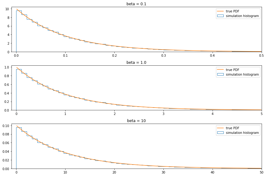
png
Exercise 3.14.16. Let \(X \sim \text{Poisson}(\lambda)\) and \(Y \sim \text{Poisson}(\mu)\) and assume that \(X\) and \(Y\) are independent. Show that the distribution of \(X\) given that \(X + Y = n\) is \(\text{Binomial}(n, \pi)\) where \(\pi = \lambda / (\lambda + \mu)\).
Hint 1: You may use the following fact: If \(X \sim \text{Poisson}(\lambda)\) and \(Y \sim \text{Poisson}(\mu)\), and \(X\) and \(Y\) are independent, then \(X + Y \sim \text{Poisson}(\mu + \lambda)\).
Hint 2: Note that \(\{X = x, X + Y = n\} = \{X = x, Y = n - x \}\)
Solution.
We have:
\[ \begin{align} \mathbb{P}(X = x | X + Y = n) &= \frac{\mathbb{P}(X = x, X + Y = n)}{\mathbb{P}(X + Y = n)} \\ &= \frac{\mathbb{P}(X = x, Y = n - x)}{\mathbb{P}(X + Y = n)} \\ &= \frac{\mathbb{P}(X = x) \mathbb{P}(Y = n - x)}{\mathbb{P}(X + Y = n)} \\ &= \frac{\frac{\lambda^x e^{-\lambda}}{x!} \frac{\mu^{n - x} e^{-\mu}}{(n - x)!} }{\frac{(\lambda + \mu)^n e^{-(\lambda + \mu)}}{n!}} \\ &= \frac{n!}{x! (n - x)!} \frac{\lambda^x \mu^{n - x}}{(\lambda + \mu)^n} \\ &= \binom{n}{x} \left( \frac{\lambda}{\lambda + \mu} \right)^x \left( \frac{\mu}{\lambda + \mu}\right)^{n - x} \\ &= \binom{n}{x} \pi^x (1 - \pi)^{n - x} \end{align} \]
and so the result follows.
Exercise 3.14.17. Let
\[ f_{X, Y}(x, y) = \begin{cases} c(x + y^2) &\text{if } 0 \leq x \leq 1 \text{ and } 0 \leq y \leq 1 \\ 0 & \text{otherwise} \end{cases} \]
Find \(\mathbb{P}\left( X < \frac{1}{2} | Y = \frac{1}{2} \right)\).
Solution.
The conditional density \(f_{X | Y}(x | y)\) is:
\[ f_{X|Y}(x | y) = \frac{f_{X, Y}(x, y)}{f_Y(y)} = \frac{f_{X, Y}(x, y)}{\int f_{X, Y}(t, y) dt} = \frac{ c(x + y^2) }{\int_0^1 c(t + y^2) dt} = \frac{ x + y^2 }{\int_0^1 t + y^2 dt} = \frac{x + y^2}{\frac{1}{2} + y^2} \]
In particular, when \(y = 1/2\),
\[f_{X|Y}(x | 1/2) = \frac{4x + 1}{3}\]
and so
\[ \mathbb{P}\left( X < x \;\Bigg|\; Y = \frac{1}{2} \right) = \int_0^x \frac{4t + 1}{3} dt = \frac{2x^2 + x}{3} \]
so
\[ \mathbb{P}\left( X < \frac{1}{2} \;\Bigg|\; Y = \frac{1}{2} \right) = \frac{1}{3} \]
Exercie 3.14.18. Let \(X \sim N(3, 16)\). Solve the following using the Normal table and using a computer package.
(a) Find \(\mathbb{P}(X < 7)\).
(b) Find \(\mathbb{P}(X > -2)\).
(c) Find \(x\) such that \(\mathbb{P}(X > x) = .05\).
(d) Find \(\mathbb{P}(0 \leq X < 4)\).
(e) Find \(x\) such that \(\mathbb{P}(|X| > |x|) = .05\).
Solution.
Rather than using tables, we will express these in terms of a standard Normal, and use “computer packages” to compute the expression based both on the original Normal and the standard Normal.
(a) \(\mathbb{P}(X < 7) = \mathbb{P}\left(\frac{X - 3}{16} < \frac{7 - 3}{16} \right) = \mathbb{P}\left(Z < \frac{1}{4} \right) = \Phi\left( \frac{1}{4} \right)\)
import numpy as np
from scipy.stats import norm

print('%.4f' % norm.cdf(1/4))
print('%.4f' % norm.cdf(7, loc=3, scale=16))
0.5987
0.5987(b) $(X > -2) = ( > ) = (Z < - ) = 1 - ( - ) $
import numpy as np
from scipy.stats import norm

print('%.4f' % (1 - norm.cdf(-5/16)))
print('%.4f' % (1 - norm.cdf(-2, loc=3, scale=16)))
0.6227
0.6227(c) \[\mathbb{P}(X > x) = .05 \Longleftrightarrow 1 - F_X(x) = .05 \Longleftrightarrow F_X(x) = .95 \Longleftrightarrow x = F_X^{-1}(.95)\]
or: \[\mathbb{P}(X > x) = .05 \Longleftrightarrow \mathbb{P}\left(\frac{X - 3}{16} > \frac{x - 3}{16}\right) = .05 \Longleftrightarrow 1 - \Phi\left(\frac{x - 3}{16}\right) = .05 \Longleftrightarrow \frac{x - 3}{16} = \Phi^{-1}(.95) \Longleftrightarrow x = 16 \Phi^{-1}(.95) + 3 \]
import numpy as np
from scipy.stats import norm

print('%.4f' % norm.ppf(.95, loc=3, scale=16))
print('%.4f' % (16 * norm.ppf(.95) + 3))
29.3177
29.3177(d) \(\mathbb{P}(0 \leq X < 4) = F_X(4) - F_X(0)\)
or \(\mathbb{P}(0 \leq X < 4) = \mathbb{P}\left(\frac{0 - 3}{16} < Z < \frac{4 - 3}{16} \right) = \Phi\left( \frac{1}{16} \right) - \Phi\left( \frac{-3}{16} \right)\)
import numpy as np
from scipy.stats import norm

print('%.4f' % (norm.cdf(4, loc=3, scale=16) - norm.cdf(0, loc=3, scale=16)))
print('%.4f' % (norm.cdf(1/16) - norm.cdf(-3/16)))
0.0993
0.0993(e) \(\mathbb{P}(|X| > |x|) = .05\)
For a constant \(c \geq 0\), we have
\[ \begin{align} \mathbb{P}(|X| > c) &= 1 - \mathbb{P}(|X| < c) = 1 - \mathbb{P}(-c < X < -c) \\ &= 1 - \mathbb{P}\left( -\frac{c - 3}{16} < Z < \frac{c - 3}{16} \right)\\ &= 1 - \Phi\left( \frac{c - 3}{16} \right) + \Phi\left( -\frac{c - 3}{16} \right) \\ &= 2 - 2 \Phi\left( \frac{c - 3}{16} \right) = 2 - 2 F_X(c) \end{align} \]
So we can solve the original equation:
\[ 2 - 2 F_X(c) = .05 \Longleftrightarrow c = F_X^{-1}(0.975) \]
or
\[ 2 - 2 \Phi\left( \frac{c - 3}{16} \right) = .05 \Longleftrightarrow c = 16 \Phi^{-1}(0.975) + 3 \]
import numpy as np
from scipy.stats import norm

print('%.4f' % (norm.ppf(0.975, loc=3, scale=16)))
print('%.4f' % (16 * norm.ppf(0.975) + 3))
34.3594
34.3594Exercise 3.14.19. Prove formula (3.11).
Given \(Y = r(X)\), when \(r\) is strictly monotone increasing or strictly monotone decreasing then \(r\) has an inverse \(s = r^{-1}\) and in this case one can show that
\[ f_Y(y) = f_X(s(y)) \;\Bigg| \frac{ds(y)}{dy} \Bigg|\]
Solution.
Assume \(r\) is strictly monotone increasing. Then $ > 0$, and the CDF of \(Y\) is
\[ F_Y(y) = \mathbb{P}(Y \leq y) = \mathbb{P}(r(X) \leq y) = \mathbb{P}(X \leq s(y)) = F_X(s(y)) \]
Derivating over \(y\),
\[ \begin{align} \frac{d}{dy} F_y(y) &= \frac{d F_X(s(y))}{d s(y)} \frac{d s(y)}{dy} \\ f_Y(y) &= f_X(s(y)) \frac{d s(y)}{dy} \end{align} \]
For the case when \(r\) is strictly monotone decreasing, $ < 0$, and the CDF of \(Y\) is
\[ F_Y(y) = \mathbb{P}(Y \leq y) = \mathbb{P}(r(X) \leq y) = \mathbb{P}(X \geq s(y)) = 1 - F_X(s(y)) \]
Derivating over \(y\),
\[ \begin{align} \frac{d}{dy} F_y(y) &= \frac{d -F_X(s(y))}{d s(y)} \frac{d s(y)}{dy} \\ f_Y(y) &= -f_X(s(y)) \frac{d s(y)}{dy} \end{align} \]
and the result follows.
Exercise 3.14.20. Let \(X, Y \sim \text{Uniform}(0, 1)\) be independent. Find the PDF for \(X - Y\) and \(X / Y\).
Solution.
The joint density of \(X, Y\) is
\[ f(x, y) = \begin{cases} 1 &\text{if } 0 \leq x \leq 1, 0 \leq y \leq 1 \\ 0 &\text{otherwise} \end{cases} \]
Let \(A = X - Y\). The CDF of \(A\) is calculated over the area \(A_a = \{ (x, y) : x - y \leq a \}\):
\[ F_A(a) = \mathbb{P}(X + Y \leq a) = \int_{A_a} f(x, y)\; dx dy \]
If \(0 \leq a \leq 1\), the area is consists of all points in the unit square, othe than the triangle at points \((a, 0), (1, 0), (1, 1 - a)\). Then,
\[ F_A(a) = 1 - \frac{(1 - a)^2}{2} \]
If \(-1 \leq a \leq 0\), the area consists of only the points in the triangle \((0, 1), (1 + a, 1), (0, -a)\). Then,
\[ F_A(a) = \frac{(1 + a)^2}{2} \]
Therefore, the PDF is \(f_A(a) = F'_A(a)\), or
\[ f_A(a) = \begin{cases} 1 + a &\text{if } -1 < a \leq 0 \\ 1 - a &\text{if } 0 < a \leq 1 \\ 0 &\text{otherwise} \end{cases} \]
import numpy as np
import matplotlib.pyplot as plt
%matplotlib inline

plt.figure(figsize=(8, 4))

ax = plt.subplot(1, 2, 1)
a = 1/3
x = [0, a, 1, 1, 0]
y = [0, 0, 1 - a, 1, 1]
ax.fill(x, y)
ax.set_xlim(-0.5, 1.5)
ax.set_ylim(-0.5, 1.5)
ax.set_title('a = 1/3')

ax = plt.subplot(1, 2, 2)
a = -1/3
x = [0, 1+a, 0]
y = [1, 1, -a]
ax.fill(x, y)
ax.set_xlim(-0.5, 1.5)
ax.set_ylim(-0.5, 1.5)
ax.set_title('a = -1/3')

plt.tight_layout()
plt.show()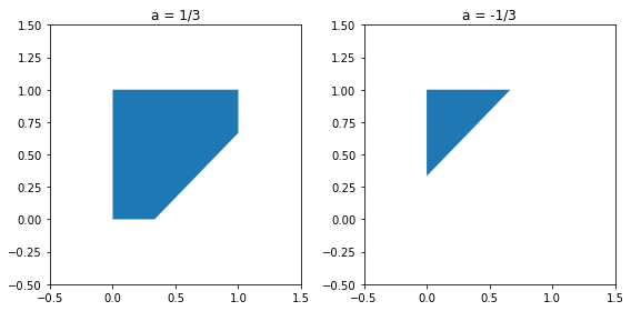
png
Let \(B = X/Y\). The CDF of \(B\) is calculated over the area \(B_b = \left\{ (x, y) : \frac{x}{y} \leq b \right\}\).
\[ F_B(a) = \mathbb{P}\left(\frac{X}{Y} \leq b\right) = \int_{B_b} f(x, y)\; dx dy \]
If \(0 < b \leq 1\), the relevant area is a triangle with points \((0, 0), (1, 0), (1, b)\). Then,
\[ F_B(b) = \frac{b}{2} \]
If \(b > 1\), the relevant area is the unit square minus the triangle with points \((0, 0), (0, 1), (1/b, 1)\). Then,
\[ F_B(b) = 1 - \frac{1}{2b} \]
Therefore, the PDF is \(f_B(b) = F'_B(b)\), or
\[ f_A(a) = \begin{cases} \frac{1}{2} &\text{if } 0 < b \leq 1 \\ \frac{1}{2b^2} &\text{if } b > 1 \\ 0 &\text{otherwise} \end{cases} \]
import numpy as np
import matplotlib.pyplot as plt
%matplotlib inline

plt.figure(figsize=(8, 4))

ax = plt.subplot(1, 2, 1)
b = 1/3
x = [0, 1, 1]
y = [0, 0, b]
ax.fill(x, y)
ax.set_xlim(-0.5, 1.5)
ax.set_ylim(-0.5, 1.5)
ax.set_title('b = 1/3')

ax = plt.subplot(1, 2, 2)
b = 3
x = [0, 1, 1, 0, 1/b]
y = [0, 0, 1, 1, 1]
ax.fill(x, y)
ax.set_xlim(-0.5, 1.5)
ax.set_ylim(-0.5, 1.5)
ax.set_title('b = 3')

plt.tight_layout()
plt.show()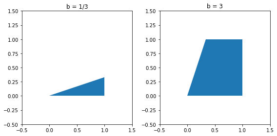
png
Exercise 3.14.21. Let \(X_1, \dots, X_n \sim \text{Exp}(\beta)\) be IID. Let \(Y = \max \{ X_1, \dots, X_n \}\). Find the PDF of \(Y\). Hint: \(Y \leq y\) if and only if \(X_i \leq y\) for \(i = 1, \dots, n\).
Solution. We have:
\[ \mathbb{P}(Y \leq y) = \mathbb{P}(\forall i, X_i \leq y) = \prod_i \mathbb{P}(X_i \leq y) = \prod_i \left(1 - e^{-y/\beta}\right) = (1 - e^{-y/\beta})^n \]
and so the PDF is \(f_Y(y) = F'_Y(y)\):
\[ f_Y(y) = \frac{d (1 - e^{-y/\beta})^n}{dy} = \frac{n}{\beta} e^{-x/\beta} (1 - e^{-x/\beta})^{n-1}\]
Exercise 3.14.22. Let \(X\) and \(Y\) be random variables. Suppose that \(\mathbb{E}(Y | X) = X\). Show that \(\text{Cov}(X, Y) = \mathbb{V}(X)\).
Solution.
The covariance is:
\[ \text{Cov}(X, Y) = \mathbb{E}(XY) - \mathbb{E}(X) \mathbb{E}(Y) \]
and the variance is
\[ \mathbb{V}(X) = \mathbb{E}(X^2) - \mathbb{E}(X)^2 \]
We aim to prove that both of those expressions have the same value when \(\mathbb{E}(Y | X) = X\).
Taking the expectaion on \(\mathbb{E}(Y | X)\) we get:
\[ \mathbb{E}(\mathbb{E}(Y | X)) = \int \mathbb{E}(Y = y | X) f_Y(y) \; dy = \int y f_Y(y) = \mathbb{E}(Y) \]
so taking the expectation on both sides of \(\mathbb{E}(Y | X) = X\) gives us \(\mathbb{E}(Y) = \mathbb{E}(X)\).
Now, we have
\[ \begin{align} \mathbb{E}(XY) &= \int \mathbb{E}(XY | X = x) f_X(x) dx \\ &= \int \mathbb{E}(xY | X = x) f_X(x) dx \\ &= \int x \mathbb{E}(Y | X = x) f_X(x) dx \\ &= \int x^2 f_X(x) dx \\ &= \mathbb{E}(X^2) \end{align} \]
Using \(\mathbb{E}(X^2) = \mathbb{E}(XY)\) and \(\mathbb{E}(Y) = \mathbb{E}(X)\), we get the desired result.
Exercise 3.14.23. Let \(X \sim \text{Uniform}(0, 1)\). Let \(0 < a < b < 1\). Let
\[ Y = \begin{cases} 1 &\text{if } 0 < x < b \\ 0 &\text{otherwise} \end{cases} \]
and let
\[ Z = \begin{cases} 1 &\text{if } a < x < 1 \\ 0 &\text{otherwise} \end{cases} \]
(a) Are \(Y\) and \(Z\) independent? Why / Why not?
(b) Find \(\mathbb{E}(Y | Z)\). Hint: what values \(z\) can \(Z\) take? Now find \(\mathbb{E}(Y | Z = z)\).
Solution.
(a) The joint probability mass function for \(Y\) and \(Z\) is:
\[ \begin{array}{c|cc} & Z = 0 & Z = 1 \\ \hline Y = 0 & 0 & 1 - b \\ Y = 1 & a & b - a \end{array} \]
These are not independent; in particular,
\[ \mathbb{P}(Y = 1, Z = 1) = b - a \neq \mathbb{P}(Y = 1) \mathbb{P}(Z = 1) = b(1 - a) \]
since the equality would only hold if \(b = 0\) or \(a = 0\), and the inequality precludes both of these.
(b) We have:
\[ \mathbb{E}(Y | Z = 0) = \frac{\sum_y y f(y, 0)}{f_Z(0)} = \frac{f(1, 0)}{a} = 1 \]
and
\[ \mathbb{E}(Y | Z = 1) = \frac{\sum_y y f(y, 1)}{f_Z(1)} = \frac{f(1, 1)}{1 - a} = \frac{b - a}{1 - a} \]