- Ex. 3.9 (using the QR decomposition for fast forward-stepwise selection)
- Ex. 3.10 (using the z-scores for fast backwards stepwise regression)
- Ex. 3.11 (multivariate linear regression with different \(\Sigma_i\))
- Ex. 3.12 (ordinary least squares to implement ridge regression)
- Ex. 3.13 (principal component regression)
- Ex. 3.14 (when the inputs are orthogonal PLS stops after m = 1 step)
- Ex. 3.15 (PLS seeks directions that have high variance and high correlation)
- Ex. 3.16 (explicit expressions for \(\hat\beta_j\) when the features are orthonormal)
- Ex. 3.17 (linear methods on the spam data set)
- Ex. 3.18 (conjugate gradient methods)
- Ex. 3.19 (increasing norm with decreasing \(\lambda\))
- Ex. 3.20
- Ex. 3.21
- Ex. 3.22
- Ex. 3.23 (\((X^TX)^{−1}X^Tr\) keeps the correlations tied and decreasing)
- Ex. 3.24 LAR directions.
- Ex. 3.25 LAR look-ahead.
- Ex. 3.26 (forward stepwise regression vs. LAR)
- Ex. 3.27 Lasso and LAR
- Ex. 3.28
- Ex. 3.29
- Ex. 3.30 (solving the elastic net optimization problem with the lasso)
- References
options(width = 300)Ex. 3.9 (using the QR decomposition for fast forward-stepwise selection)
Forward stepwise regression. Suppose we have the \(QR\) decomposition for the \(N\times q\) matrix \(X_1\) in a multiple regression problem with response \(y\), and we have an additional \(p−q\) predictors in the matrix \(X_2\). Denote the current residual by \(r\). We wish to establish which one of these additional variables will reduce the residual-sum-of squares the most when included with those in \(X_1\). Describe an efficient procedure for doing this.
Since \[\underset{N\times q}{X_1}=\underset{N\times N}{Q}\underset{N\times q}{R}\], If \(N\ge q\), \[\underset{N\times q}{X_1}=\underset{N\times N}{Q}\underset{N\times q}{R}=\begin{bmatrix} \underset{N\times q}{Q_1} & \underset{N\times (N-q)}{Q_2} \end{bmatrix}\begin{bmatrix} \underset{q\times N}{R_1} \\ \underset{(N-q)\times N}{\mathbf 0} \end{bmatrix}=\begin{bmatrix} \underset{N\times q}{Q_1} & \underset{N\times (N-q)}{Q_2} \end{bmatrix}\begin{bmatrix} \underset{q\times q}{R_2} & \underset{q\times (N-q)}{\mathbf 0}\\ \underset{(N-q)\times q}{\mathbf 0} & \underset{(N-q)\times (N-q)}{\mathbf 0}\\ \end{bmatrix}\] where \(Q_1\) and \(Q_2\) both have orthogonal columns. Each column of \(X_1\) is \[x_j=Qr_j\]. \[\hat{y}=X_1(X_1^TX_1)^{-1}X_1^Ty=QR(R^TQ^TQR)^{-1}R^TQ^Ty\\ =Q_1R_2R_2^{-1}R_2^{-T}R_2^TQ_1^Ty=Q_1Q_1^Ty\] Let the \(i\)-th column is \(Q\) is \(q_i,\quad (1\le i\le q)\), then \((q_1,\cdots,q_q)\) is an orthonormal basis of \(Q\) or \(Q_1\), then the best estimator is \[\underset{i}{\text{argmax }}(q_i^Ty)q_i\]
Ex. 3.10 (using the z-scores for fast backwards stepwise regression)
Backward stepwise regression. Suppose we have the multiple regression fit of \(y\) on \(X\), along with the standard errors and Z-scores as in Table 3.2. We wish to establish which variable, when dropped, will increase the residual sum-of-squares the least. How would you do this?
The F statistic, \[ F_{p_1−p_0,N−p_1−1}=\frac{\left(\text{RSS}_0-\text{RSS}_1\right)/\left(p_1-p_0\right)}{\text{RSS}_1/\left(N-p_1-1\right)} \] where \(\text{RSS}_1\) is the residual sum-of-squares for the least squares fit of the bigger model with \(p_1+1\) parameters, and \(\text{RSS}_0\) the same for the nested smaller model with \(p_0+1\) parameters, having \(p_1−p_0\) parameters constrained to be zero. The \(F\) statistic measures the change in residual sum-of-squares per additional parameter in the bigger model, and it is normalized by an estimate of \(\sigma^2\). Under the Gaussian assumptions, and the null hypothesis that the smaller model is correct, the \(F\) statistic will have a \(F_{p_1−p_0,N−p_1−1}\) distribution.
The \(Z-score\) \[z_j=\frac{\hat{\beta}_j}{\hat{\sigma}\sqrt{v_{jj}}}\] where \(v_{jj}\) is the \(j\)th diagonal element of \((\mathbf X^T\mathbf X)^{−1}\). Under the null hypothesis that \(\beta_j = 0\), \(z_j\) is distributed as \(t_{N−p−1}\) (a \(t\) distribution with \(N − p − 1\) degrees of freedom), and hence a large (absolute) value of \(z_j\) will lead to rejection of this null hypothesis.
Since once \(\beta\) is estimated we can compute \(\sigma^2\): \[\hat{\sigma}^2=\frac{1}{N-p-1}\sum_{i=1}^{N}(y_i-\hat{y}_i)^2=\frac{1}{N-p-1}\sum_{i=1}^{N}(y_i-x_i^T\beta)^2=\frac{\text{RSS}_1}{N-p-1}\] In addition, by just deleting one variable from our regression the difference in degrees of freedom between the two models is one i.e. \(p_1 − p_0 = 1\). Thus the \(F\)-statistic when we delete the \(j\)th term from the base model simplifies to \[F_{1,N−p_1−1}=\frac{\left(\text{RSS}_j-\text{RSS}_1\right)}{\text{RSS}_1/\left(N-p_1-1\right)}=\frac{\left(\text{RSS}_j-\text{RSS}_1\right)}{\hat{\sigma}^2}\]
Since \[\text{RSS}_j-\text{RSS}_1=\left(\mathbf{y'}-\mathbf{X'}\left(\mathbf{X'}^T\mathbf{X'}\right)^{-1}\mathbf{X'}^T\mathbf{y'}\right)^T\left(\mathbf{y'}-\mathbf{X'}\left(\mathbf{X'}^T\mathbf{X'}\right)^{-1}\mathbf{X'}^T\mathbf{y'}\right)-\left(\mathbf{y}-\mathbf{X}\left(\mathbf{X}^T\mathbf{X}\right)^{-1}\mathbf{X}^T\mathbf{y}\right)^T\left(\mathbf{y}-\mathbf{X}\left(\mathbf{X}^T\mathbf{X}\right)^{-1}\mathbf{X}^T\mathbf{y}\right)\] Where \(\mathbf{X'}\) is \(\mathbf{X}\) with \(j\)th column deleted and \(\mathbf{y'}\) is \(\mathbf{y}\) with \(j\)th element deleted.
Since that \(X^TX(X^TX)^{−1} = I_{p+1}\). Let \(u_j\) be the \(jth\) column of \(X(X^TX)^{−1}\). Using the \(v_{ij}\) notation to denote the elements of the matrix \((X^TX)^{−1}\) established above, we have \[u_j=\sum_{r=1}^{p+1}x_rv_{rj}\] and \[\lVert u_j\rVert^2=u_j^Tu_j=\sum_{r=1}^{p+1}v_{rj}x_r^Tu_j=\sum_{r=1}^{p+1}v_{rj}x_r^Tu_j=v_{jj}\] Then \[\lVert z_j\rVert^2=\frac{\lVert u_j\rVert^2}{v_{jj}^2}=\frac{1}{v_{jj}}\] Now \[\frac{z_j}{\lVert z_j\rVert}\] is a unit vector orthogonal to \(x_1, \cdots , x_{j−1}, x_{j+1}, \cdots , x_{p+1}\). So \[\text{RSS}_j-\text{RSS}_1=\left<y,\frac{z_j}{\lVert z_j\rVert}\right>^2=\left(\frac{<y,z_j>}{<z_j,z_j>}\right)^2\lVert z_j\rVert^2=\hat{\beta}_j^2/v_{jj}\] and \[F_{1,N−p_1−1}=\frac{\left(\text{RSS}_j-\text{RSS}_1\right)}{\text{RSS}_1/\left(N-p_1-1\right)}=\frac{\left(\text{RSS}_j-\text{RSS}_1\right)}{\hat{\sigma}^2}=\frac{\hat{\beta}_j^2}{\hat{\sigma}^2v_{jj}}=z_j^2\]
Ex. 3.11 (multivariate linear regression with different \(\Sigma_i\))
Show that the solution to the multivariate linear regression problem (3.40) is given by (3.39). What happens if the covariance matrices \(\mathbf\Sigma_i\) are different for each observation?
\[\begin{align} \text{RSS}(\mathbf{B}) &= \sum_{k=1}^K \sum_{i=1}^N \left( y_{ik} - f_k(x_i) \right)^2 \\ &= \text{trace}\left( (\mathbf{Y}-\mathbf{XB})^T(\mathbf{Y}-\mathbf{XB}) \right) \end{align}\quad(Equation\;\;3.38)\] \[\begin{equation} \hat{\mathbf{B}} = \left(\mathbf{X}^T\mathbf{X}\right)^{-1}\mathbf{X}^T\mathbf{Y}. \end{equation}\quad(Equation\;\;3.39)\] \[\begin{equation} \text{RSS}(\mathbf{B};\mathbf{\Sigma}) = \sum_{i=1}^N (y_i-f(x_i))^T \mathbf{\Sigma}^{-1} (y_i-f(x_i)) \end{equation} \quad(Equation\;\;3.40)\]
With \(N\) training cases we can write the model in matrix notation \[ \begin{equation} \mathbf{Y}=\mathbf{XB}+\mathbf{E}, \end{equation} \] where
- \(\mathbf{Y}\) is \(N\times K\) with \(ik\) entry \(y_{ik}\),
- \(\mathbf{X}\) is \(N\times(p+1)\) input matrix,
- \(\mathbf{B}\) is \((p+1)\times K\) parameter matrix,
- \(\mathbf{E}\) is \(N\times K\) error matrix.
A straightforward generalization of the univariate loss function is \[ \begin{align} \text{RSS}(\mathbf{B}) &= \sum_{k=1}^K \sum_{i=1}^N \left( y_{ik} - f_k(x_i) \right)^2 \\ &= \text{trace}\left( (\mathbf{Y}-\mathbf{XB})^T(\mathbf{Y}-\mathbf{XB}) \right) \end{align}\]
The least squares estimates have exactly the same form as before \[ \begin{equation} \hat{\mathbf{B}} = \left(\mathbf{X}^T\mathbf{X}\right)^{-1}\mathbf{X}^T\mathbf{Y}. \end{equation} \quad(Equation\;\;3.39)\]
If the errors \(\epsilon = (\epsilon_1,\cdots,\epsilon_K)\) are correlated with \(\text{Cov}(\epsilon)=\mathbf{\Sigma}\), then the multivariate weighted criterion \[ \begin{equation} \text{RSS}(\mathbf{B};\mathbf{\Sigma}) = \sum_{i=1}^N (y_i-f(x_i))^T \mathbf{\Sigma}^{-1} (y_i-f(x_i)) \end{equation} \quad(Equation\;\;3.40)\]
if the covariance matrices \(\mathbf\Sigma_i\) are different for each observation \[ \begin{equation} \text{RSS}(\mathbf{B}) = \sum_{i=1}^N (y_i-f(x_i))^T \mathbf{\Sigma_i}^{-1} (y_i-f(x_i)) \end{equation}\]
Ex. 3.12 (ordinary least squares to implement ridge regression)
Show that the ridge regression estimates can be obtained by ordinary least squares regression on an augmented data set. We augment the centered matrix \(X\) with \(p\) additional rows \(\sqrt{\lambda}\mathbf I\), and augment \(y\) with \(p\) zeros. By introducing artificial data having response value zero, the fitting procedure is forced to shrink the coefficients toward zero. This is related to the idea of hints due to Abu-Mostafa (1995), where model constraints are implemented by adding artificial data examples that satisfy them.
Consider the input centered data matrix \(\mathbf X\) (of size \(p\times p\)) and the output data vector \(\mathbf Y\) both appended (to produce the new variables \(\hat{\mathbf X}\) and \(\hat{\mathbf Y}\) ) as follows \[\hat{\mathbf X}=\begin{bmatrix} \underset{p\times p}{\mathbf X}\\ \sqrt{\lambda}\underset{p\times p}{\mathbf I}\\ \end{bmatrix}\] and \[\hat{\mathbf Y}=\begin{bmatrix} \underset{p\times 1}{\mathbf Y}\\ \underset{p\times 1}{\mathbf 0}\\ \end{bmatrix}\] The the classic least squares solution to this new problem is given by \[ \begin{align} \hat{\mathbf{\beta^{ls}}} &= \left(\mathbf{\hat X}^T\mathbf{\hat X}\right)^{-1}\mathbf{\hat X}^T\mathbf{\hat Y}\\ &=\left(\begin{bmatrix} \underset{p\times p}{\mathbf X}^T&\sqrt{\lambda}\underset{p\times p}{\mathbf I}^T\\ \end{bmatrix}\begin{bmatrix} \underset{p\times p}{\mathbf X}\\ \sqrt{\lambda}\underset{p\times p}{\mathbf I}\\ \end{bmatrix}\right)^{-1}\begin{bmatrix} \underset{p\times p}{\mathbf X}^T&\sqrt{\lambda}\underset{p\times p}{\mathbf I}^T\\ \end{bmatrix}\begin{bmatrix} \underset{p\times 1}{\mathbf Y}\\ \underset{p\times 1}{\mathbf 0}\\ \end{bmatrix}\\ &=\left(\mathbf X^T\mathbf X+\lambda\mathbf I\right)^{-1}\left(\mathbf X^T\mathbf Y\right) \end{align} \] This expression we recognize as the solution to the regularized least squares proving the equivalence.
Ex. 3.13 (principal component regression)
Derive the expression (3.62), and show that \[\hat{\beta}^{pcr}(p)=\hat{β}^{ls}\]
The linear combinations \(Z_m\) used in principal component regression (PCR) are the principal components. PCR forms the derived input columns \[ \begin{equation} \mathbf{z}_m = \mathbf{X} v_m, \end{equation} \] and then regress \(\mathbf{y}\) on \(\mathbf{z}_1,\mathbf{z}_2,\cdots,\mathbf{z}_M\) for some \(M\le p\). Since the \(\mathbf{z}_m\) are orthogonal, this regression is just a sum of univariate regressions: \[ \begin{equation} \hat{\mathbf{y}}_{(M)}^{\text{pcr}} = \bar{y}\mathbf{1} + \sum_{m=1}^M \hat\theta_m \mathbf{z}_m = \bar{y}\mathbf{1} + \mathbf{X}\mathbf{V}_M\hat{\mathbf{\theta}}=\bar{y}\mathbf{1} + \mathbf{X}\sum_{m=1}^M\hat\theta_mv_m, \end{equation} \]
where \(\hat\theta_m = \langle\mathbf{z}_m,\mathbf{y}\rangle \big/ \langle\mathbf{z}_m,\mathbf{z}_m\rangle\). We can see from the last equality that, since the \(\mathbf{z}_m\) are each linear combinations of the original \(\mathbf{x}_j\), we can express the solution in terms of coefficients of the \(\mathbf{x}_j\). \[\begin{bmatrix} \mathbf 1 &\mathbf X \end{bmatrix}\] and \[ \begin{equation} \hat\beta^{\text{pcr}}(M) = \begin{bmatrix} \bar{y}\\ \sum_{m=1}^M \hat\theta_m v_m \end{bmatrix} \end{equation} \quad(Equation\;\;3.62) \]
For multiple linear regression models the estimated regression coefficients in the vector \(\hat{\beta}\) can be split into two parts a scalar \(\hat\beta_0\) and a \(p \times 1\) vector \(\hat\beta^∗\) as \[\hat{\beta}=\begin{bmatrix} \hat\beta_0\\ \hat\beta^∗ \end{bmatrix}\] In addition the coefficient \(\hat\beta_0\) can be shown to be related to \(\hat\beta^∗\) as\[\hat\beta_0=\bar{y}-\hat\beta^∗\bar{x}\] and since \[\begin{bmatrix} \bar{y}\\ \sum_{m=1}^M \hat\theta_m v_m \end{bmatrix}=\begin{bmatrix} \hat\beta_0\\ \hat\beta^∗ \end{bmatrix}\] then \(\hat\beta_0=\bar{y}\) and \(\bar{x}=0\), which means in in principal component regression, the input predictor variables are standardized.
To evaluate \(\hat\beta^{\text{pcr}}(M)\) when \(M = p\), recall that in principal component regression the vectors \(v_m\) are from the \(SVD\) decomposition of the matrix \(X\) given by \(X = UDV^T\). This later expression is equivalent to \(XV = UD\) from which we get \[ \begin{align} Xv_1&=d_1u_1\\ Xv_2&=d_2u_2\\ \vdots\\ Xv_p&=d_pu_p\\ \end{align}\] Since the vectors \(z_m\) are given by \(z_m = Xv_m\) for \(1 \le m \le M \le p\), by the above we have the vectors \(z_m\) in terms of the vectors \(u_m\) as \(z_m = d_mu_m\). Since for this problem we are to show that when \(M = p\) the estimate \(\hat\beta^{\text{pcr}}(M)\) above becomes the least squares estimate \(\hat\beta^{\text{ls}}\) When \(\lambda = 0\) the ridge regression estimate for \(\beta\) is equal to the least squares estimate (when \(\lambda = 0\) we have no \(\lambda\lVert\beta\rVert_2^2\) ridge penalty term) we can use Equation \[ \begin{align} \hat\beta^{\text{ridge}} &= \left( \mathbf{X}^T\mathbf{X} + \lambda\mathbf{I} \right)^{-1}\mathbf{X}^T\mathbf{y}\\ &=(\mathbf V\mathbf D^2\mathbf V^T+\lambda\mathbf{V}\mathbf{V}^T)^{-1}\mathbf V\mathbf D\mathbf U^T\mathbf{y}\\ &=(\mathbf V(\mathbf D^2+\lambda\mathbf{I})\mathbf{V}^T)^{-1}\mathbf V\mathbf D\mathbf U^T\mathbf{y}\\ &=\mathbf{V}^{-T}(\mathbf D^2+\lambda\mathbf{I})^{-1}\mathbf D\mathbf U^T\mathbf{y}\\ &=\mathbf{V}(\mathbf D^2+\lambda\mathbf{I})^{-1}\mathbf D\mathbf U^T\mathbf{y}\\ \end{align} \] to obtain \[\hat\beta^{\text{ls}}=\hat\beta^{\text{ridge}}(\lambda=0)=\mathbf{V}\mathbf D^{-2}\mathbf D\mathbf U^T\mathbf{y}\\=\mathbf{V}\mathbf D^{-1}\mathbf U^T\mathbf{y}\] Since \[\hat\beta^{\text{pcr}}(p)=\sum_{m=1}^M\hat\theta_mv_m=\mathbf{V}\begin{bmatrix} \hat\theta_1\\ \hat\theta_2\\ \vdots\\ \hat\theta_p \end{bmatrix}=\mathbf{V}\begin{bmatrix} \langle\mathbf{z}_1,\mathbf{y}\rangle \big/ \langle\mathbf{z}_1,\mathbf{z}_1\rangle\\ \langle\mathbf{z}_2,\mathbf{y}\rangle \big/ \langle\mathbf{z}_2,\mathbf{z}_2\rangle\\ \vdots\\ \langle\mathbf{z}_p,\mathbf{y}\rangle \big/ \langle\mathbf{z}_p,\mathbf{z}_p\rangle \end{bmatrix}\] and since \(z_m = d_mu_m\) we have \[\langle\mathbf{z}_m,\mathbf{z}_m\rangle=d_m^2\langle\mathbf{u}_m,\mathbf{u}_m\rangle=d_m^2\] since the vectors \(u_m\) are assumed to be orthonormal. Also \(\langle\mathbf{z}_m,\mathbf{y}\rangle = d_m \langle\mathbf{u}_m,\mathbf{y}\rangle\), so the estimate for \[\hat\beta^{\text{pcr}}(p)=\mathbf{V}\begin{bmatrix} \langle\mathbf{z}_1,\mathbf{y}\rangle \big/ \langle\mathbf{z}_1,\mathbf{z}_1\rangle\\ \langle\mathbf{z}_2,\mathbf{y}\rangle \big/ \langle\mathbf{z}_2,\mathbf{z}_2\rangle\\ \vdots\\ \langle\mathbf{z}_p,\mathbf{y}\rangle \big/ \langle\mathbf{z}_p,\mathbf{z}_p\rangle \end{bmatrix}=\mathbf{V}\begin{bmatrix} \langle\mathbf{u}_1,\mathbf{y}\rangle \big/ d_1\\ \langle\mathbf{u}_1,\mathbf{y}\rangle \big/ d_1\\ \vdots\\ \langle\mathbf{u}_1,\mathbf{y}\rangle \big/ d_1\\ \end{bmatrix}=\mathbf{V}\mathbf D^{-1}\mathbf U^T\mathbf{y}\\ =\hat\beta^{\text{ls}}=\hat\beta^{\text{ridge}}(\lambda=0)\]
Ex. 3.14 (when the inputs are orthogonal PLS stops after m = 1 step)
Show that in the orthogonal case, \(\text{PLS}\) stops after \(m = 1\) steps, because subsequent \(\hat{\varphi}_{mj}\) in step 2 in Algorithm 3.3 are zero.
Algorithm 3.3 Partial Least Squares:
Standardize each \(x_j\) to have mean zero and variance one. Set \(\hat y^{(0)} =\bar{y}\mathbf 1\), and \(x^{(0)}_j = x_j , j = 1, \cdots, p\).
For \(m=1,2,\cdots,p\)
\[z_m=\sum_{j=1}^{p}\hat\varphi_{mj}x_j^{(m-1)}\] where \[\hat\varphi_{mj}=\langle x_j^{(m-1)}, y\rangle\]
\[\hat\theta_m=\langle z_m, y\rangle\big/\langle z_m, z_m\rangle\]
\[\hat{y}^{(m)}=\hat{y}^{(m-1)}+\hat\theta_mz_m\]
Orthogonalize each \(x_j^{(m-1)}\) with respect to \[z_m:x_j^{(m)}=x_j^{(m-1)}-\left[\langle z_m, x_j^{(m-1)}\rangle\big/\langle z_m, z_m\rangle\right]z_m, j=1,2,\cdots,p\]
- Output the sequence of fitted vectors \(\{\hat y^{(m)}\}_1^p\). Since the \(\{z_{\ell}\}_1^m\) are linear in the original \(x_j\), so is \(\hat y^{(m)} = X\hat{\beta}^{\text{pls}}(m)\). These linear coefficients can be recovered from the sequence of \(\text{PLS}\) transformations.
In Algorithm 3.3 on partial least squares (PLS) if on any given step \(m\) we compute that \[\hat\varphi_{mj} =\langle x_j^{(m-1)}, y\rangle= 0\] for all \(j\) then all \[z_m=\sum_{j=1}^{p}\hat\varphi_{mj}x_j^{(m-1)}=0\] it follows that the algorithm must stop. If the \(x_j\)’s are orthogonal, we have
\[z_1=\sum_{j=1}^{p}\hat\varphi_{1j}x_j^{(0)}\] where \[\hat\varphi_{1j}=\langle x_j^{(0)}, y\rangle\]
\[\hat\theta_1=\langle z_1, y\rangle\big/\langle z_1, z_1\rangle\] Since \[\begin{align} \langle z_1, z_1\rangle&=\left\langle \sum_{j=1}^{p}\hat\varphi_{1j}x_j^{(0)}, \sum_{j=1}^{p}\hat\varphi_{1j}x_j^{(0)}\right\rangle\\ &=\sum_{j=1}^{p}\sum_{j'=1}^{p}\hat\varphi_{1j}\hat\varphi_{1j'}\left\langle x_j^{(0)},x_{j'}^{(0)}\right\rangle\\ &=\sum_{j=1}^{p}\hat\varphi_{1j}^2\\ \end{align}\] since the vectors \(x_j^{(0)}\) are orthogonal. \[\langle z_1, y\rangle=\left\langle \sum_{j=1}^{p}\hat\varphi_{1j}x_j^{(0)}, y\right\rangle=\sum_{j=1}^{p}\hat\varphi_{1j}\left\langle x_j^{(0)}, y\right\rangle=\sum_{j=1}^{p}\hat\varphi_{1j}^2\] and thus we have \[\hat\theta_1=\langle z_1, y\rangle\big/\langle z_1, z_1\rangle=1\]
\[\hat{y}^{(1)}=\hat{y}^{(0)}+\hat\theta_1z_1=\hat{y}^{(0)}+z_1=\hat{y}^{(0)}+\sum_{j=1}^{p}\hat\varphi_{1j}x_j^{(0)}\]
Orthogonalize each \(x_j^{(1)}, j=1,2,\cdots,p\) with respect to \[z_1:x_j^{(1)}=x_j^{(0)}-\left[\langle z_1, x_j^{(0)}\rangle\big/\langle z_1, z_1\rangle\right]z_1\] Since the vectors \(x^{(0)}_j\) are orthogonal \[\langle z_1, x_k^{(0)}\rangle=\sum_{j=1}^{p}\hat\varphi_{1j}\langle x_j^{(0)}, x_k^{(0)}\rangle=\hat\varphi_{1k}\] then \[\begin{align} x_j^{(1)}&=x_j^{(0)}-\left[\langle z_1, x_j^{(0)}\rangle\big/\langle z_1, z_1\rangle\right]z_1\\ &=x_j^{(0)}-\left[\hat\varphi_{1j}\big/\sum_{j=1}^{p}\hat\varphi_{1j}^2\right]\sum_{j=1}^{p}\hat\varphi_{1j}x_j^{(0)}\\ \end{align}\] Having finished the first loop of Algorithm 3.3 we let \(m = 2\) and compute \(\hat\varphi_{2j}\) to get \[\hat\varphi_{2j}=\langle x_j^{(1)}, y\rangle=\langle x_j^{(0)}, y\rangle-\left[\hat\varphi_{1j}\big/\sum_{j=1}^{p}\hat\varphi_{1j}^2\right]\sum_{j=1}^{p}\hat\varphi_{1j}^2\\ =\hat\varphi_{1j}-\hat\varphi_{1j}=0\]
Ex. 3.15 (PLS seeks directions that have high variance and high correlation)
Verify expression (3.64), and hence show that the partial least squares directions are a compromise between the ordinary regression coefficient and the principal component directions.
PLS begins by computing the weights \[ \begin{equation} \hat\varphi_{1j} = \langle \mathbf{x}_j,\mathbf{y} \rangle, \text{ for each } j, \end{equation} \] which are in fact the univariate regression coefficients, since \(\mathbf{x}_j\) are standardized (only for the first step \(m=1\)).
From this we construct derived input \[ \begin{equation} \mathbf{z}_1 = \sum_j \hat\varphi_{1j}\mathbf{x}_j, \end{equation} \] which is the first PLS direction. Hence in the construction of each \(\mathbf{z}_m\), the inputs are weighted by the strength of their univariate effect on \(\mathbf{y}\).
The outcome \(\mathbf{y}\) is regressed on \(\mathbf{z}_1\) giving coefficient \(\hat\theta_1\), and then we orthogonalize \(\mathbf{x}_1,\cdots,\mathbf{x}_p\) w.r.t. \(\mathbf{z}_1\).
We continue this process, until \(M\le p\) directions have been obtained. In this manner, PLS produces a sequence of derived, orthogonal inputs or directions \(\mathbf{z}_1,\cdots,\mathbf{z}_M\).
- As with PCR, if \(M=p\), then \(\hat\beta^{\text{pls}} = \hat\beta^{\text{ls}}\).
- Using \(M<p\) directions produces a reduced regression.
Relation to the optimization problem
PLS seeks direction that have high variance and have high correlation with the response, in contrast to PCR with keys only on high variance (Stone and Brooks, 1990; Frank and Friedman, 1993). Since it uses the response \(\mathbf{y}\) to construct its directions, its solution path is a nonlinear function of \(\mathbf{y}\).
In particular, the \(m\)th principal component direction \(v_m\) solves: \[ \begin{equation} \max_\alpha \text{Var}(\mathbf{X}\alpha)\\ \text{subject to } \|\alpha\| = 1, \alpha^T\mathbf{S} v_l = 0 \text{ for } l = 1,\cdots, m-1, \end{equation} \] where \(\mathbf{S}\) is the sample covariance matrix of the \(\mathbf{x}_j\). The condition \(\alpha^T\mathbf{S} v_l= 0\) ensures that \(\mathbf{z}_m = \mathbf{X}\alpha\) is uncorrelated with all the previous linear combinations \(\mathbf{z}_l = \mathbf{X} v_l\).
The \(m\)th PLS direction \(\hat\varphi_m\) solves: \[ \begin{equation} \max_\alpha \text{Corr}^2(\mathbf{y},\mathbf{S}\alpha)\text{Var}(\mathbf{X}\alpha)\\ \text{subject to } \|\alpha\| = 1, \alpha^T\mathbf{S}\hat\varphi_l = 0, \text{ for } l=1,\cdots, m-1. \end{equation} \quad (3.64) \]
Ex. 3.16 (explicit expressions for \(\hat\beta_j\) when the features are orthonormal)
Derive the entries in Table 3.4, the explicit forms for estimators in the orthogonal case.
TABLE 3.4. Estimators of \(\beta_j\) in the case of orthonormal columns of \(\mathbf X\). \(M\) and \(\lambda\) are constants chosen by the corresponding techniques; sign denotes the sign of its argument (\(\pm 1\)), and \(x_+\) denotes “positive part” of \(x\). Below the table, estimators are shown by broken red lines. The \(45^\circ\) line in gray shows the unrestricted estimate for reference.
\[\begin{array}{l} \text{Estimator} & \text{Formula}\\ \hline \text{Best subset (size M)} &\hat{\beta}_j\cdot I(\lvert\hat{\beta}_j\rvert\ge\lvert\hat{\beta}_{(M)}\rvert)\\ \text{Ridge} & \hat{\beta}_j\big/(1+\lambda)\\ \text{Lasso} & \text{sign}(\hat{\beta}_j)(\lvert\hat{\beta}_j\rvert-\lambda)_+\\ \hline \end{array}\] When the predictors are orthonormal \(X^TX = I\) and the ordinary least squared estimate of \(\beta\) is given by \[\hat\beta=X^TY\]
In best-subset selection we will take the top \(M\) predictors that result in the smallest residual sum of squares. Since the columns of \(X\) are orthonormal we can construct a basis for \(\mathbb R^N\) by using the first \(p\) columns of \(X\) and then extending these with \(N −p\) linearly independent additional orthonormal vectors. The Gram-Schmidt procedure guarantees that we can do this. Thus in this extended basis we can write \(y\) as \[y=\sum_{j=1}^{p}\hat\beta_jx_j+\sum_{j=p+1}^{N}\gamma_j\tilde{x}_j\] where \(\hat\beta_j\) equal the components of \(\hat\beta\) in \[\hat\beta=X^TY\] \(\tilde{x}_j\) are the extended basis vectors required to span \(\mathbb R^N\), and \(\gamma_j\) are the coefficients of \(y\) with respect to these extended basis vectors. Then if we seek to approximate \(y\) with a subset of size \(M\) as in best subset selection, \(\hat y\) can be written as \[\hat y=\sum_{j=1}^{p}I_j\hat\beta_jx_j\] with \(I_j=1\) if we keep the predictor \(x_j\) and zero otherwise. Now since all the vectors \(x_j\) and \(\tilde{x}_j\) are orthonormal we have \[\begin{align} \lVert y-\hat y\rVert_2^2&=\lVert y-X\hat\beta\rVert_2^2\\ &=\left\lVert \sum_{j=1}^{p}\hat\beta_jx_j+\sum_{j=p+1}^{N}\gamma_j\tilde{x}_j-X\hat\beta\right\rVert_2^2\\ &=\left\lVert \sum_{j=1}^{p}\hat\beta_j(\mathbf 1-I_j)x_j+\sum_{j=p+1}^{N}\gamma_j\tilde{x}_j\right\rVert_2^2\\ &=\sum_{j=1}^{p}\hat\beta_j^2(\mathbf 1-I_j)^2\left\lVert x_j\right\rVert_2^2+\sum_{j=p+1}^{N}\gamma_j^2\left\lVert\tilde{x}_j\right\rVert_2^2\\ &=\sum_{j=1}^{p}\hat\beta_j^2(\mathbf 1-I_j)^2+\sum_{j=p+1}^{N}\gamma_j^2\\ \end{align}\]
Thus to minimize \(\lVert y-\hat y\rVert_2^2\) we would pick the \(M\) values of \(I_j\) to be equal to one that have the largest \(\beta_j^2\) values. This is equivalent to sorting the values \(\lvert\hat\beta_j\rvert\) and picking the indices of the largest \(M\) of these to have \(I_j = 1\). All other indices \(j\) would be taken to have \(I_j = 0\). Using an indicator function this is equivalent to the expression \[\hat\beta_j^{\text{best subset}}=\hat\beta_j\cdot I\left( \lvert\hat\beta_j\rvert \ge \lvert\hat\beta_{(M)}\rvert \right)\]
- Best subset (size \(M\)) drops all variables with coefficients smaller than the \(M\)th largest; this is a form of “hard-thresholding.”
\[\begin{equation} \hat\beta_j\cdot I\left( \lvert\hat\beta_j\rvert \ge \lvert\hat\beta_{(M)}\rvert \right) \end{equation}\]
For ridge regression, since \(X\) has orthonormal columns we have \[\begin{align} \hat\beta^{\text{ridge}}&= \left( \mathbf{X}^T\mathbf{X} + \lambda I \right)^{-1}\mathbf{X}^T\mathbf{y}\\ &=\left( I + \lambda I \right)^{-1}\mathbf{X}^T\mathbf{y}\\ &=\frac{\mathbf{X}^T\mathbf{y}}{1+\lambda}\\ &=\frac{\hat\beta^{\text{ls}}}{1+\lambda} \end{align}\] * Ridge does a proportional shrinkage.
\[\begin{equation} \frac{\hat\beta_j}{1+\lambda} \end{equation}\]
The lasso estimate is defined by \[\begin{equation} \hat\beta^{\text{lasso}} = \arg\min_\beta \left\lbrace \frac{1}{2}\sum_{i=1}^N \left( y_i-\beta_0-\sum_{j=1}^p x_{ij}\beta_j \right)^2 + \lambda\sum_{j=1}^p |\beta_j| \right\rbrace, \end{equation}\] For the lasso regression procedure we pick the values of \(\beta_j\) to minimize \[\text{RSS}(\beta)=\frac{1}{2}(y-X\beta)^T(y-X\beta)+\lambda\sum_{j=1}^{p}\lvert \beta_j\rvert\] Expanding \(\hat y\) as \[\hat y = \sum_{j=1}^{p} \beta_jx_j\] and with \[y=\sum_{j=1}^{p}\hat\beta_jx_j+\sum_{j=p+1}^{N}\gamma_j\tilde{x}_j\] we have that \(\text{RSS}(\beta)\) in this case becomes \[\begin{align} \text{RSS}(\beta)&=\frac{1}{2}\left\lVert \sum_{j=1}^{p}(\hat\beta_j-\beta_j)x_j+\sum_{j=p+1}^{N}\gamma_j\tilde{x}_j\right\rVert_2^2+\lambda\sum_{j=1}^{p}\lvert \beta_j\rvert\\ &=\frac{1}{2}\sum_{j=1}^{p}(\hat\beta_j-\beta_j)^2+\frac{1}{2}\sum_{j=p+1}^{N}\gamma_j^2+\lambda\sum_{j=1}^{p}\lvert \beta_j\rvert\\ &=\frac{1}{2}\sum_{j=1}^{p}\left[(\hat\beta_j-\beta_j)^2+2\lambda\lvert \beta_j\rvert\right]+\sum_{j=p+1}^{N}\gamma_j^2 \end{align}\] We can minimize this expression for each value of \(\beta_j\) for \(1 \le j \le p\) independently. Thus our vector problem becomes that of solving \(p\) scalar minimization problems all of which look like \[\beta^*=\text{argmin}_{\beta}\left[(\hat\beta-\beta)^2+2\lambda\lvert \beta\rvert\right]\] Then the objective function we want to minimize is \[ F(\beta)=\begin{cases} (\hat\beta-\beta)^2-2\lambda\beta &\text{ when } \beta<0\\[2ex] (\hat\beta-\beta)^2+2\lambda\beta &\text{ when } \beta>0\\ \end{cases} \] where \(\hat\beta\) is the least squares estimate.
To find the minimum of this function take the derivative with respect to \(\beta\) and set the result equal to zero and solve for \(\beta\). We find the derivative of \(F(\beta)\) given by \[ F'(\beta)=\begin{cases} 2(\beta-\hat\beta)-2\lambda &\text{ when } \beta<0\\[2ex] 2(\beta-\hat\beta)+2\lambda &\text{ when } \beta>0\\ \end{cases} \] When we set \(F'(\beta)\) equal to zero we get two possible solutions for \(\beta\) given by \[\begin{cases} \beta=+\lambda+\hat\beta &\text{ when } \beta<0\\[2ex] \beta=-\lambda+\hat\beta &\text{ when } \beta>0\\[2ex] \end{cases}\]
- Lasso translates each coefficient by a constant factor \(\lambda\), truncating at zero. This is called “soft-thresholding.”
\[\begin{equation} \text{sign}\left( \hat\beta_j \right)\left( \lvert\hat\beta_j\rvert - \lambda \right)_+ \end{equation}\]
In this expression \(\hat\beta\) and \(\lambda\) are assumed fixed.
%load_ext rpy2.ipython%%R
xx = seq(-15,+15,length=1000) # the range of beta's to sample
# the specific parameters:
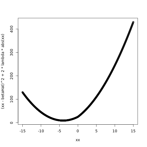
betaHat = -5.0
lambda = 1.0
plot( xx, ( xx - betaHat )^2 + 2*lambda*abs(xx) )
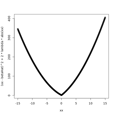
betaHat = -1.0
lambda = 5.0
plot( xx, ( xx - betaHat )^2 + 2*lambda*abs(xx) )
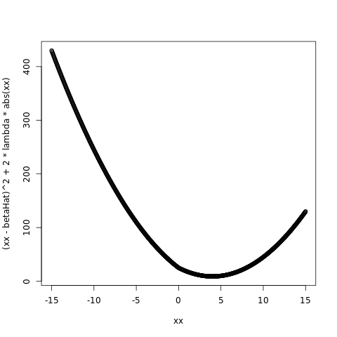
betaHat = 5.0
lambda = 1.0
plot( xx, ( xx - betaHat )^2 + 2*lambda*abs(xx) )
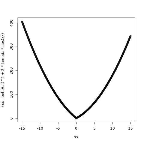
betaHat = 1.0
lambda = 5.0
plot( xx, ( xx - betaHat )^2 + 2*lambda*abs(xx) )
png
png
png
png
Ex. 3.17 (linear methods on the spam data set)
Repeat the analysis of Table 3.3 on the spam data discussed in Chapter 1.
%%R
load_spam_data <- function(trainingScale=TRUE,responseScale=TRUE){

  X      = read.table("../../data/Spam/spam.data.txt")
  tt     = read.table("../../data/Spam/spam.traintest.txt")

  # separate into training/testing sets

  XTraining = subset( X, tt==0 )
  p = dim(XTraining)[2]-1

  XTesting  = subset( X, tt==1 )

  #
  # Sometime data is processed and stored in a certain order.  When doing cross validation
  # on such data sets we don't want to bias our results if we grab the first or the last samples.
  # Thus we randomize the order of the rows in the Training data frame to make sure that each
  # cross validation training/testing set is as random as possible.
  #
  if( FALSE ){
    nSamples = dim(XTraining)[1]
    inds = sample( 1:nSamples, nSamples )
    XTraining = XTraining[inds,]
  }

  #
  # In reality we have to estimate everything based on the training data only
  # Thus here we estimate the predictor statistics using the training set
  # and then scale the testing set by the same statistics
  #
  if( trainingScale ){
    X = XTraining
    if( responseScale ){
      meanV58 = mean(X$V58)
      v58 = X$V58 - meanV58
    }else{
      v58 = X$V58
    }
    X$V58 = NULL
    X = scale(X, TRUE, TRUE)
    means = attr(X,"scaled:center")
    stds = attr(X,"scaled:scale")
    Xf = data.frame(X)
    Xf$V58 = v58
    XTraining = Xf

    # scale the testing predictors by the same amounts:
    #
    DCVTest  = XTesting
    if( responseScale ){
      v58Test = DCVTest$V58 - meanV58
    }else{
      v58Test = DCVTest$V58 # in physical units (not mean adjusted)
    }
    DCVTest$V58 = NULL
    DCVTest  = t( apply( DCVTest, 1, '-', means ) )
    DCVTest  = t( apply( DCVTest, 1, '/', stds ) )
    DCVTestb = cbind( DCVTest, v58Test ) # append back on the response
    DCVTestf = data.frame( DCVTestb ) # a data frame containing all scaled variables of interest
    names(DCVTestf)[p+1] = "V58" # fix the name of the response
    XTesting = DCVTestf
  }

  # Many algorithms wont do well if the data is presented all of one class and
  # then all of another class thus we permute our data frames :
  #
  XTraining = XTraining[sample(nrow(XTraining)),]
  XTesting  = XTesting[sample(nrow(XTesting)),]

  # Read in the list of s(pam)words (and delete garbage characters):
  #
  spam_words = read.table("../../data/Spam/spambase.names",skip=33,sep=":",comment.char="|",stringsAsFactors=F)
  spam_words = spam_words[[1]]
  for( si in 1:length(spam_words) ){
    spam_words[si] = sub( "word_freq_", "", spam_words[si] )
    spam_words[si] = sub( "char_freq_", "", spam_words[si] )
  }

  return( list( XTraining, XTesting, spam_words ) )
}
OLS:
%%R
res = load_spam_data(trainingScale=TRUE,responseScale=FALSE)
XTraining = res[[1]]
XTesting = res[[2]]

nrow = dim( XTraining )[1]
p = dim( XTraining )[2] - 1 # the last column is the response

D = XTraining[,1:p] # get the predictor data

# Append a column of ones:
#
Dp = cbind( matrix(1,nrow,1), as.matrix( D ) )

response = XTraining[,p+1]

library(MASS)

betaHat = ginv( t(Dp) %*% Dp ) %*% t(Dp) %*% as.matrix(response)

# this is basically the first column in Table 3.2:
#


# make predictions based on these estimated beta coefficients:
#
yhat = Dp %*% betaHat

# estimate the variance:
#
sigmaHat = sum( ( response - yhat )^2 ) / ( nrow - p - 1 )

# calculate the covariance of betaHat:
#
covarBetaHat = sigmaHat * ginv( t(Dp) %*% Dp )

# calulate the standard deviations of betahat:
#
stdBetaHat = sqrt(diag(covarBetaHat))

# this is basically the second column in Table 3.2:
#


# compute the z-scores:
#
z = betaHat / stdBetaHat

# this is basically the third column in Table 3.2:
#


cbind(data.frame(`beta estimates` = betaHat), data.frame(`beta standard errors` = as.matrix(stdBetaHat)), data.frame(`beta z-scores` = z))

# display the results we get :
F = data.frame( Term=c("Intercept",names(XTraining)[1:p]), Coefficients=betaHat, Std_Error=stdBetaHat, Z_Score=z )
library(xtable)
xtable( F, caption="Table of OLS coefficients for the SPAM data set", digits=2 )

# Run this full linear model on the Testing data so that we can fill in the two
# lower spots in the "LS" column in Table 3.2
#
pdt = cbind( matrix(1,dim(XTesting)[1],1), as.matrix( XTesting[,1:p] ) ) %*% betaHat
responseTest = XTesting[,p+1]
NTest = length(responseTest)
mErr = mean( (responseTest - pdt)^2 )
print( mErr )
sErr = sqrt( var( (responseTest - pdt)^2 )/NTest )
print( sErr )
[1] 0.1212304
[,1]
[1,] 0.007212358Runs ridge regression on the SPAM data set:
%%R
cv_Ridge <- function( lambda, D, numberOfCV ){
#
# Does Cross Validation of the Ridge Regression Linear Model specified by the formula "form"
#
# Input:
# lambda = multiplier of the penatly term
# D = training data frame where the last column is the response variable
# numberOfCV = number of cross validations to do
#
# Output:
# MSPE = vector of length numberOfCV with components mean square prediction errors
# extracted from each of the numberOfCV test data sets
library(MASS) # needed for ginv
nSamples = dim( D )[1]
p = dim( D )[2] - 1 # the last column is the response
# needed for the cross vaildation (CV) loops:
#
nCVTest = round( nSamples*(1/numberOfCV) ) # each CV run will have this many test points
nCVTrain = nSamples-nCVTest # each CV run will have this many training points
for (cvi in 1:numberOfCV) {
testInds = (cvi-1)*nCVTest + 1:nCVTest # this may attempt to access sample indexes > nSamples
testInds = intersect( testInds, 1:nSamples ) # so we restrict this list here
DCVTest = D[testInds,1:(p+1)] # get the predictor + response testing data
# select this cross validation's section of data from all the training data:
#
trainInds = setdiff( 1:nSamples, testInds )
DCV = D[trainInds,1:(p+1)] # get the predictor + response training data
# Get the response and delete it from the data frame
#
responseName = names(DCV)[p+1] # get the actual string name from the data frame
response = DCV[,p+1]
DCV[[responseName]] = NULL
# For ridge-regression we begin by standardizing the predictors and demeaning the response
#
# Note that one can get the centering value (the mean) with the command attr(DCV,'scaled:center')
# and the scaling value (the sample standard deviation) with the command attr(DCV,'scaled:scale')
#
DCV = scale( DCV )
responseMean = mean( response )
response = response - responseMean
DCVb = cbind( DCV, response ) # append back on the response
DCVf = data.frame( DCVb ) # a data frame containing all scaled variables of interest
# extract the centering and scaling information:
#
means = attr(DCV,"scaled:center")
stds = attr(DCV,"scaled:scale")
# apply the computed scaling based on the training data to the testing data:
#
responseTest = DCVTest[,p+1] - responseMean # mean adjust
DCVTest[[responseName]] = NULL
DCVTest = t( apply( DCVTest, 1, '-', means ) )
DCVTest = t( apply( DCVTest, 1, '/', stds ) )
DCVTestb = cbind( DCVTest, responseTest ) # append back on the response
DCVTestf = data.frame( DCVTestb ) # a data frame containing all scaled variables of interest
names(DCVTestf)[p+1] = responseName # fix the name of the response
# fit this linear model and compute the expected prediction error (EPE) using these features (this just estimates the mean in this case):
#
DM = as.matrix(DCV)
M = ginv( t(DM) %*% DM + lambda*diag(p) ) %*% t(DM)
betaHat = M %*% as.matrix(DCVf[,p+1])
DTest = as.matrix(DCVTest)
pdt = DTest %*% betaHat # get demeaned predictions on the test set
#pdt = pdt + responseMean # add back in the mean if we want the response in physical units (not mean adjusted)
if( cvi==1 ){
predmat = pdt
y = responseTest
}else{
predmat = c( predmat, pdt )
y = c( y, responseTest )
}
} # endfor cvi loop
# this code is modeled after the code in "glmnet/cvelnet.R"
#
N = length(y)
cvraw = ( y - predmat )^2
cvm = mean(cvraw)
cvsd = sqrt( var(cvraw)/N )
l = list( cvraw=cvraw, cvm=cvm, cvsd=cvsd, name="Mean Squared Error" )
return(l)
}
one_standard_error_rule <- function(complexityParam,cvResults){
#
# Input:
# complexityParam = the sampled complexity parameter (duplicate cross vaidation results expected)
# cvResults = matrix where
# each column is a different value of the complexity parameter (with complexity increasing from left to right) ...
# each row is the square prediction error (SPE) of a different cross validation sample i.e. ( y_i - \hat{y}_i )^2
#
# Output:
# optCP = the optimal complexity parameter
N = dim(cvResults)[1]
# compute the complexity based mean and standard deviations:
means = apply(cvResults,2,mean)
stds = sqrt( apply(cvResults,2,var)/N )
# find the smallest espe:
minIndex = which.min( means )
# compute the confidence interval around this point:
#cip = 1 - 2*pnorm(-1)
#ciw <- qt(cip/2, n) * stdev / sqrt(n)
ciw = stds[minIndex]
# add a width of one std to the min point:
maxUncertInMin = means[minIndex] + 0.5*ciw
# find the mean that is nearest to this value and that is a SIMPLER model than the minimum mean model:
complexityIndex = which.min( abs( means[1:minIndex] - maxUncertInMin ) )
complexityValue = complexityParam[complexityIndex]
# package everything to send out:
res = list(complexityValue,complexityIndex,maxUncertInMin, means,stds)
return(res)
}
df_ridge <- function(lambda,X){
#
# R code to compute the degress of freedom for ridge regression.
# This is formula 3.50 in the book.
#
# Input:
# lambda: the penalty term coefficent
# X the data matrix
#
# Output:
#
# dof: the degrees of freedom.
library(MASS) # needed for ginv
XTX = t(X) %*% X
pprime = dim(XTX)[1]
Hlambda = X %*% ginv( XTX + lambda * diag(pprime) ) %*% t(X)
dof = sum( diag( Hlambda ) )
return(dof)
}
opt_lambda_ridge <- function(X,multiple=1){
#
# Returns the "optimal" set of lambda for nice looking ridge regression plots.
#
# Input:
#
# X = matrix or data frame of features (do not prepend a constant of ones)
#
# Output:
# lambdas = vector of optimal lambda (choosen to make the degrees_of_freedom(lambda)
# equal to equal to the integers 1:p
#
# Notes: these values of lambda are selected to solve (equation 3.50 for various values of dof)
#
# dof = \sum_{i=1}^p \frac{ d_j^2 }{ d_j^2 + \lambda }
s = svd( X )
dj = s$d # the diagional elements d_j. Note that dj[1] is the largest value, while dj[end] is the smallest
p = dim( X )[2]
# Do degrees_of_freedom=p first (this is the value for lambda when the degrees of freedom is *p*)
lambdas = 0
# Do all other values for the degrees_of_freedom next:
#
kRange = seq(p-1,1,by=(-1/multiple) )
for( ki in 1:length(kRange) ){
# solve for lambda in (via newton iterations):
# k = \sum_{i=1}^p \frac{ d_j^2 }{ d_j^2 + \lambda }
#
k = kRange[ki]
# intialGuess at the root
if( ki==1 ){
xn = 0.0
}else{
xn = xnp1 # use the oldest previously computed root
}
f = sum( dj^2 / ( dj^2 + xn ) ) - k # do the first update by hand
fp = - sum( dj^2 / ( dj^2 + xn )^2 )
xnp1 = xn - f/fp
while( abs(xn - xnp1)/abs(xn) > 10^(-3) ){
xn = xnp1
f = sum( dj^2 / ( dj^2 + xn ) ) - k
fp = - sum( dj^2 / ( dj^2 + xn )^2 )
xnp1 = xn - f/fp
}
lambdas = c(lambdas,xnp1)
}
# flip the order of the lambdas:
lambdas = lambdas[ rev(1:length(lambdas)) ]
return(lambdas)
}
PD2 <- load_spam_data(trainingScale=FALSE,responseScale=FALSE)
XTraining = PD2[[1]]
XTesting = PD2[[2]]
p = dim(XTraining)[2]-1 # the last column is the response
nSamples = dim(XTraining)[1]
# Do ridge-regression cross validation (large lambda values => small degrees of freedom):
#
allLambdas = opt_lambda_ridge( XTraining[,1:p], multiple=2 )
numberOfLambdas = length( allLambdas )
for( li in 1:numberOfLambdas ){
res = cv_Ridge(allLambdas[li],XTraining,numberOfCV=10)
# To get a *single* value for the degrees of freedom use the call on the entire training data set
# We could also take the mean/median of this computed from the cross validation samples
#
dof = df_ridge(allLambdas[li],as.matrix(XTraining[,1:p]))
if( li==1 ){
complexityParam = dof
cvResults = res$cvraw
}else{
complexityParam = cbind( complexityParam, dof ) # will be sorted from largest value of dof to smallest valued dof
cvResults = cbind( cvResults, res$cvraw ) # each column is a different value of the complexity parameter ...
# each row is a different cross validation sample ...
}
}
# flip the order of the results:
inds = rev( 1:numberOfLambdas )
allLambdas = allLambdas[ inds ]
complexityParam = complexityParam[ inds ]
cvResults = cvResults[ , inds ]
# group all cvResults by lambda (the complexity parameter) and compute statistics:
#
OSE = one_standard_error_rule( complexityParam, cvResults )
complexVValue = OSE[[1]]
complexIndex = OSE[[2]]
oseHValue = OSE[[3]]
means = OSE[[4]] # as a function of model complexity
stds = OSE[[5]] # as a function of model complexity
library(gplots) # plotCI, plotmeans found here, xlim=c(0,8), ylim=c(0.3,1.8)
plotCI( x=complexityParam, y=means, uiw=0.5*stds,
col="black", barcol="blue", lwd=1, type="l",
xlab="degrees of freedom", ylab="expected squared prediction error (ESPE)" )
abline( h=oseHValue, lty=2 )
abline( v=complexVValue, lty=2 )
# pick the best model, retrain over the entire data set, and predict on the testing data set:
#
bestLambda = allLambdas[ complexIndex ]
DCV = XTraining
#
#
responseName = names(DCV)[p+1] # get the response and delete it from the data frame
response = DCV[,p+1]
DCV[[responseName]] = NULL
# Standardize the predictors and demean the response
#
# Note that one can get the centering value (the mean) with the command attr(DCV,'scaled:center')
# and the scaling value (the sample standard deviation) with the command attr(DCV,'scaled:scale')
#
DCV = scale( DCV )
responseMean = mean( response )
response = response - responseMean
DCVb = cbind( DCV, response ) # append back on the response
DCVf = data.frame( DCVb ) # a data frame containing all scaled variables of interest
# extract the centering and scaling information:
#
means = attr(DCV,"scaled:center")
stds = attr(DCV,"scaled:scale")
# apply the computed scaling based on the training data to the testing data:
#
DCVTest = XTesting
responseTest = DCVTest[,p+1] - responseMean # in demeaned units (not mean adjusted)
DCVTest[[responseName]] = NULL
DCVTest = t( apply( DCVTest, 1, '-', means ) )
DCVTest = t( apply( DCVTest, 1, '/', stds ) )
DCVTestb = cbind( DCVTest, responseTest ) # append back on the response
DCVTestf = data.frame( DCVTestb ) # a data frame containing all scaled variables of interest
names(DCVTestf)[p+1] = responseName # fix the name of the response
# fit this linear model and compute the expected prediction error (EPE) using these features (this just estimates the mean in this case):
#
DM = as.matrix(DCV)
M = ginv( t(DM) %*% DM + bestLambda*diag(p) ) %*% t(DM)
betaHat = M %*% as.matrix(DCVf[,p+1])
print( responseMean, digits=4 )
print( betaHat, digits=3 )
DTest = as.matrix(DCVTest)
pdt = DTest %*% betaHat # get predictions on the test set
#pdt = pdt + responseMean # add back in the mean. Now in physical units (not mean adjusted)
mErr = mean( (responseTest - pdt)^2 )
print( mErr )
NTest = length(responseTest)
sErr = sqrt( var( (responseTest - pdt)^2 )/NTest )
print( sErr )R[write to console]:
Attaching package: ‘gplots’
R[write to console]: The following object is masked from ‘package:stats’:
lowess
[1] 0.3974
[,1]
[1,] -0.012063
[2,] -0.018186
[3,] 0.024423
[4,] 0.017785
[5,] 0.048324
[6,] 0.035094
[7,] 0.082626
[8,] 0.038886
[9,] 0.012246
[10,] 0.010097
[11,] 0.008338
[12,] -0.022603
[13,] 0.000821
[14,] 0.005473
[15,] 0.008723
[16,] 0.080193
[17,] 0.025889
[18,] 0.025022
[19,] 0.033607
[20,] 0.020922
[21,] 0.063838
[22,] 0.046940
[23,] 0.058275
[24,] 0.041145
[25,] -0.041553
[26,] -0.013468
[27,] -0.036863
[28,] -0.013823
[29,] -0.002609
[30,] -0.022522
[31,] -0.004602
[32,] 0.033556
[33,] -0.017971
[34,] -0.023728
[35,] -0.009010
[36,] 0.016002
[37,] -0.009944
[38,] -0.012490
[39,] -0.017749
[40,] 0.023000
[41,] -0.001821
[42,] -0.025790
[43,] -0.012405
[44,] -0.020960
[45,] -0.039588
[46,] -0.034961
[47,] -0.009396
[48,] -0.018026
[49,] -0.030376
[50,] -0.027790
[51,] -0.004496
[52,] 0.041522
[53,] 0.061850
[54,] 0.012561
[55,] 0.005090
[56,] 0.021765
[57,] 0.038060
[1] 0.1212304
            [,1]
[1,] 0.007212358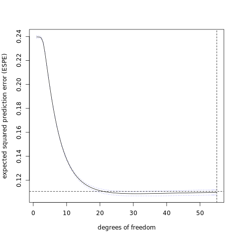
png
The lasso
%%R
PD = load_spam_data(trainingScale=TRUE,responseScale=TRUE) # read in unscaled data
XTraining = PD[[1]]
XTesting = PD[[2]]
p = dim(XTraining)[2]-1 # the last column is the response
nSamples = dim(XTraining)[1]
library(glmnet)
# alpha = 1 => lasso
fit = glmnet( as.matrix( XTraining[,1:p] ), XTraining[,p+1], family="gaussian", alpha=1 )
# alpha = 0 => ridge
#fit = glmnet( as.matrix( XTraining[,1:p] ), XTraining[,p+1], family="gaussian", alpha=0 )
#postscript("../../WriteUp/Graphics/Chapter3/spam_lasso_beta_paths.eps", onefile=FALSE, horizontal=FALSE)
plot(fit)
#dev.off()
# do crossvalidation to get the optimal value of lambda
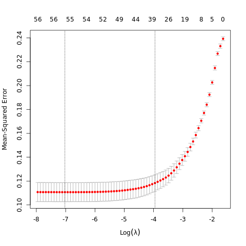
cvob = cv.glmnet( as.matrix( XTraining[,1:p] ), XTraining[,p+1], family="gaussian", alpha=1 )
#postscript("../../WriteUp/Graphics/Chapter3/spam_lasso.eps", onefile=FALSE, horizontal=FALSE)
plot( cvob )
#dev.off()
# get the optimal value of lambda:
lambdaOptimal = cvob$lambda.1se
# refit with this opimal value of lambda:
fitOpt = glmnet( as.matrix( XTraining[,1:p] ), XTraining[,p+1], family="gaussian", lambda=lambdaOptimal, alpha=1 )
print( coef(fitOpt), digit=3 )
# predict the testing data using this value of lambda:
yPredict = predict( fit, newx=as.matrix(XTesting[,1:p]), s=lambdaOptimal )
NTest = dim(XTesting[,1:p])[1]
print( mean( ( XTesting[,p+1] - yPredict )^2 ), digit=3 )
print( sqrt( var( ( XTesting[,p+1] - yPredict )^2 )/NTest ), digit=3 )
R[write to console]: Loading required package: Matrix

R[write to console]: Loaded glmnet 4.1-1


58 x 1 sparse Matrix of class "dgCMatrix"
                      s0
(Intercept)     4.69e-16
V1          .
V2          .
V3              1.60e-02
V4              2.10e-03
V5              3.88e-02
V6              3.08e-02
V7              8.27e-02
V8              3.07e-02
V9              1.11e-02
V10         .
V11             1.98e-03
V12         .
V13         .
V14         .
V15             4.26e-03
V16             7.94e-02
V17             2.32e-02
V18             1.76e-02
V19             2.99e-02
V20             1.66e-02
V21             7.37e-02
V22             2.50e-02
V23             6.02e-02
V24             3.22e-02
V25            -3.55e-02
V26            -1.38e-02
V27            -1.69e-02
V28            -2.85e-03
V29         .
V30         .
V31         .
V32         .
V33            -4.85e-03
V34         .
V35         .
V36         .
V37            -8.83e-03
V38         .
V39            -1.03e-02
V40         .
V41         .
V42            -1.54e-02
V43            -2.42e-03
V44            -3.66e-03
V45            -2.29e-02
V46            -1.87e-02
V47         .
V48            -9.88e-04
V49            -2.55e-03
V50         .
V51         .
V52             3.22e-02
V53             5.71e-02
V54         .
V55         .
V56             1.19e-03
V57             4.10e-02
[1] 0.126
        1
1 0.00708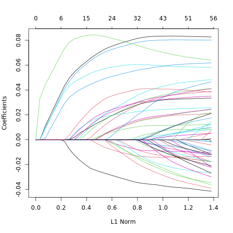
png
png
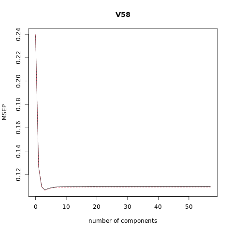
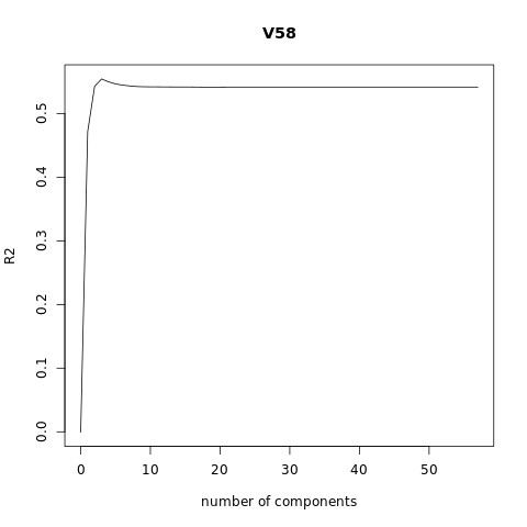
principal component regression (PCR)
%%R
require(pls)
set.seed (1000)
PD = load_spam_data(trainingScale=TRUE,responseScale=TRUE) # read in unscaled data
XTraining = PD[[1]]
XTesting = PD[[2]]
p = dim(XTraining)[2]-1 # the last column is the response
nSamples = dim(XTraining)[1]
pcr_model <- pcr(V58~., data = XTraining, scale = FALSE, validation = "CV")
summary(pcr_model)
# Plot the root mean squared error
validationplot(pcr_model)
# Plot the cross validation MSE
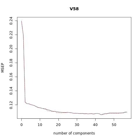
validationplot(pcr_model, val.type="MSEP")
# Plot the R2
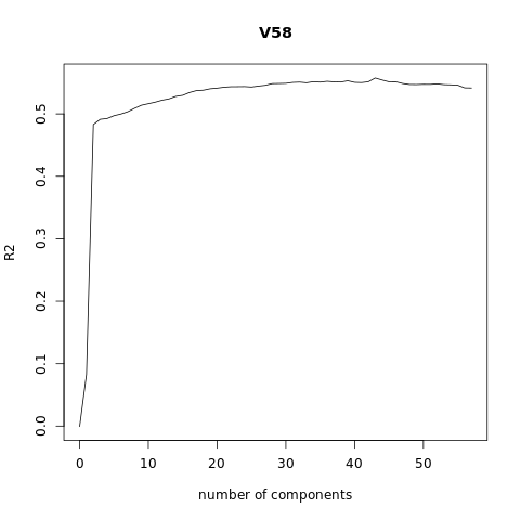
validationplot(pcr_model, val.type = "R2")
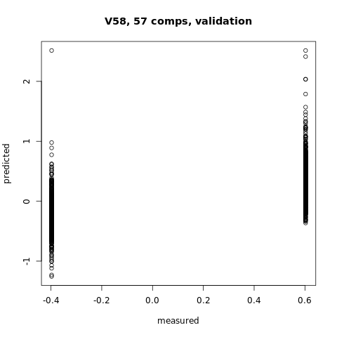
#You can plot the predicted vs measured values using the predplot function as below
predplot(pcr_model)
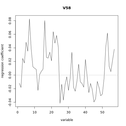
#while the regression coefficients can be plotted using the coefplot function
coefplot(pcr_model)
set.seed(777)
yPredict<-predict(pcr_model,as.matrix(XTesting[,1:p]),ncomp=20)
NTest = dim(XTesting[,1:p])[1]
print( mean( ( XTesting[,p+1] - yPredict )^2 ), digit=3 )
print( sqrt( var( ( XTesting[,p+1] - yPredict )^2 )/NTest ), digit=3 )
R[write to console]: Loading required package: pls

R[write to console]:
Attaching package: ‘pls’


R[write to console]: The following object is masked from ‘package:stats’:

    loadings


Data:   X dimension: 3065 57
    Y dimension: 3065 1
Fit method: svdpc
Number of components considered: 57

VALIDATION: RMSEP
Cross-validated using 10 random segments.
       (Intercept)  1 comps  2 comps  3 comps  4 comps  5 comps  6 comps
CV          0.4895   0.4687   0.3519   0.3490   0.3486   0.3470   0.3461
adjCV       0.4895   0.4688   0.3511   0.3488   0.3490   0.3469   0.3461
       7 comps  8 comps  9 comps  10 comps  11 comps  12 comps  13 comps
CV      0.3448   0.3429   0.3412    0.3403    0.3394    0.3383    0.3376
adjCV   0.3451   0.3423   0.3406    0.3408    0.3393    0.3391    0.3387
       14 comps  15 comps  16 comps  17 comps  18 comps  19 comps  20 comps
CV       0.3362    0.3356    0.3339    0.3328    0.3326    0.3318    0.3314
adjCV    0.3340    0.3332    0.3326    0.3323    0.3326    0.3300    0.3299
       21 comps  22 comps  23 comps  24 comps  25 comps  26 comps  27 comps
CV       0.3309    0.3306    0.3306    0.3305    0.3308    0.3302    0.3298
adjCV    0.3293    0.3294    0.3298    0.3299    0.3302    0.3305    0.3298
       28 comps  29 comps  30 comps  31 comps  32 comps  33 comps  34 comps
CV       0.3288    0.3287    0.3286    0.3281    0.3279    0.3283    0.3277
adjCV    0.3286    0.3289    0.3289    0.3282    0.3283    0.3283    0.3272
       35 comps  36 comps  37 comps  38 comps  39 comps  40 comps  41 comps
CV       0.3279    0.3274    0.3278    0.3279    0.3271    0.3281    0.3282
adjCV    0.3276    0.3272    0.3278    0.3274    0.3266    0.3278    0.3281
       42 comps  43 comps  44 comps  45 comps  46 comps  47 comps  48 comps
CV       0.3277    0.3255    0.3267    0.3277    0.3277    0.3287    0.3293
adjCV    0.3279    0.3253    0.3260    0.3272    0.3272    0.3281    0.3287
       49 comps  50 comps  51 comps  52 comps  53 comps  54 comps  55 comps
CV       0.3294    0.3292    0.3292    0.3290    0.3294    0.3295    0.3297
adjCV    0.3287    0.3286    0.3287    0.3283    0.3288    0.3289    0.3290
       56 comps  57 comps
CV       0.3313    0.3314
adjCV    0.3305    0.3306

TRAINING: % variance explained
     1 comps  2 comps  3 comps  4 comps  5 comps  6 comps  7 comps  8 comps
X     11.932    17.76    21.39    24.23    27.01    29.67    32.14    34.60
V58    8.719    47.40    48.93    48.98    49.56    49.88    50.09    50.72
     9 comps  10 comps  11 comps  12 comps  13 comps  14 comps  15 comps
X      36.93     39.20     41.41     43.42     45.41     47.37     49.29
V58    51.29     51.39     51.90     51.91     52.05     53.28     53.54
     16 comps  17 comps  18 comps  19 comps  20 comps  21 comps  22 comps
X       51.16     52.98     54.78     56.55     58.32     60.06     61.79
V58     53.74     53.78     53.81     54.49     54.51     54.74     54.82
     23 comps  24 comps  25 comps  26 comps  27 comps  28 comps  29 comps
X       63.48     65.14     66.78     68.38     69.95     71.52     73.05
V58     54.83     54.86     54.95     54.96     55.13     55.32     55.32
     30 comps  31 comps  32 comps  33 comps  34 comps  35 comps  36 comps
X       74.54     75.97     77.40     78.78     80.12     81.44     82.74
V58     55.50     55.72     55.79     56.01     56.23     56.24     56.35
     37 comps  38 comps  39 comps  40 comps  41 comps  42 comps  43 comps
X       84.02     85.26     86.47     87.66     88.83     89.96     91.02
V58     56.39     56.56     56.69     56.69     56.77     56.81     57.23
     44 comps  45 comps  46 comps  47 comps  48 comps  49 comps  50 comps
X       92.07     93.06     94.04     94.96     95.81     96.55     97.27
V58     57.45     57.46     57.51     57.57     57.57     57.58     57.61
     51 comps  52 comps  53 comps  54 comps  55 comps  56 comps  57 comps
X       97.86     98.42     98.97     99.38     99.73    100.00    100.00
V58     57.63     57.67     57.68     57.69     57.70     57.71     57.71
[1] 0.124
[1] 0.00633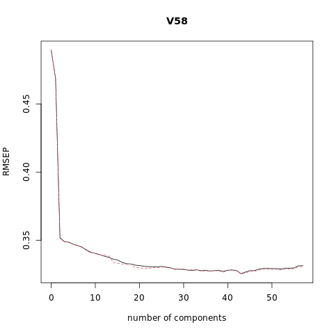
png
png
png
png

png
partial least squares regression (PLS)
%%R
require(pls)
set.seed (1000)

PD = load_spam_data(trainingScale=TRUE,responseScale=TRUE) # read in unscaled data

XTraining = PD[[1]]
XTesting = PD[[2]]

p        = dim(XTraining)[2]-1 # the last column is the response
nSamples = dim(XTraining)[1]

plsr_model <- plsr(V58~., data = XTraining, scale = FALSE, validation = "CV")
summary(plsr_model)
# Plot the root mean squared error
validationplot(plsr_model)
# Plot the cross validation MSE
validationplot(plsr_model, val.type="MSEP")
# Plot the R2
validationplot(plsr_model, val.type = "R2")

#You can plot the predicted vs measured values using the predplot function as below
predplot(plsr_model)

#while the regression coefficients can be plotted using the coefplot function
coefplot(plsr_model)

set.seed(777)
yPredict<-predict(plsr_model,as.matrix(XTesting[,1:p]),ncomp=4)

NTest = dim(XTesting[,1:p])[1]
print( mean( ( XTesting[,p+1] - yPredict )^2 ), digit=3 )
print( sqrt( var( ( XTesting[,p+1] - yPredict )^2 )/NTest ), digit=3 )
Data: X dimension: 3065 57
Y dimension: 3065 1
Fit method: kernelpls
Number of components considered: 57
VALIDATION: RMSEP
Cross-validated using 10 random segments.
(Intercept) 1 comps 2 comps 3 comps 4 comps 5 comps 6 comps
CV 0.4895 0.3558 0.3309 0.3267 0.3284 0.3296 0.3303
adjCV 0.4895 0.3557 0.3309 0.3263 0.3279 0.3289 0.3296
7 comps 8 comps 9 comps 10 comps 11 comps 12 comps 13 comps
CV 0.3307 0.3311 0.3312 0.3312 0.3313 0.3313 0.3313
adjCV 0.3299 0.3303 0.3304 0.3304 0.3304 0.3305 0.3305
14 comps 15 comps 16 comps 17 comps 18 comps 19 comps 20 comps
CV 0.3313 0.3313 0.3313 0.3314 0.3314 0.3314 0.3314
adjCV 0.3305 0.3305 0.3305 0.3306 0.3306 0.3306 0.3306
21 comps 22 comps 23 comps 24 comps 25 comps 26 comps 27 comps
CV 0.3314 0.3314 0.3314 0.3314 0.3314 0.3314 0.3314
adjCV 0.3306 0.3306 0.3306 0.3306 0.3306 0.3306 0.3306
28 comps 29 comps 30 comps 31 comps 32 comps 33 comps 34 comps
CV 0.3314 0.3314 0.3314 0.3314 0.3314 0.3314 0.3314
adjCV 0.3306 0.3306 0.3306 0.3306 0.3306 0.3306 0.3306
35 comps 36 comps 37 comps 38 comps 39 comps 40 comps 41 comps
CV 0.3314 0.3314 0.3314 0.3314 0.3314 0.3314 0.3314
adjCV 0.3306 0.3306 0.3306 0.3306 0.3306 0.3306 0.3306
42 comps 43 comps 44 comps 45 comps 46 comps 47 comps 48 comps
CV 0.3314 0.3314 0.3314 0.3314 0.3314 0.3314 0.3314
adjCV 0.3306 0.3306 0.3306 0.3306 0.3306 0.3306 0.3306
49 comps 50 comps 51 comps 52 comps 53 comps 54 comps 55 comps
CV 0.3314 0.3314 0.3314 0.3314 0.3314 0.3314 0.3314
adjCV 0.3306 0.3306 0.3306 0.3306 0.3306 0.3306 0.3306
56 comps 57 comps
CV 0.3314 0.3314
adjCV 0.3306 0.3306
TRAINING: % variance explained
1 comps 2 comps 3 comps 4 comps 5 comps 6 comps 7 comps 8 comps
X 8.668 17.38 19.94 22.60 24.80 26.64 28.11 29.74
V58 47.367 54.82 57.36 57.63 57.69 57.70 57.70 57.70
9 comps 10 comps 11 comps 12 comps 13 comps 14 comps 15 comps
X 31.23 32.56 34.18 35.81 37.28 38.87 40.34
V58 57.71 57.71 57.71 57.71 57.71 57.71 57.71
16 comps 17 comps 18 comps 19 comps 20 comps 21 comps 22 comps
X 41.85 43.10 44.22 45.78 47.25 48.53 49.74
V58 57.71 57.71 57.71 57.71 57.71 57.71 57.71
23 comps 24 comps 25 comps 26 comps 27 comps 28 comps 29 comps
X 51.24 52.90 54.18 55.49 57.19 58.58 59.95
V58 57.71 57.71 57.71 57.71 57.71 57.71 57.71
30 comps 31 comps 32 comps 33 comps 34 comps 35 comps 36 comps
X 61.25 62.53 63.74 64.95 66.33 67.65 69.00
V58 57.71 57.71 57.71 57.71 57.71 57.71 57.71
37 comps 38 comps 39 comps 40 comps 41 comps 42 comps 43 comps
X 70.50 72.02 73.58 74.98 76.48 77.90 79.31
V58 57.71 57.71 57.71 57.71 57.71 57.71 57.71
44 comps 45 comps 46 comps 47 comps 48 comps 49 comps 50 comps
X 80.65 82.00 83.50 84.94 86.48 88.05 89.63
V58 57.71 57.71 57.71 57.71 57.71 57.71 57.71
51 comps 52 comps 53 comps 54 comps 55 comps 56 comps 57 comps
X 91.21 92.79 94.37 95.94 97.52 99.10 100.68
V58 57.71 57.71 57.71 57.71 57.71 57.71 57.71
[1] 0.121
[1] 0.00748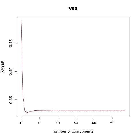
png
png
png

png
png
Ex. 3.18 (conjugate gradient methods)
Read about conjugate gradient algorithms (Murray et al., 1981, for example), and establish a connection between these algorithms and partial least squares.
The conjugate gradient method is an algorithm that can be adapted to find the minimum of nonlinear functions. It also provides a way to solve certain linear algebraic equations of the type \(Ax = b\) by formulating them as a minimization problem. Since the least squares solution \(\hat\beta\) is given by the solution of a quadratic minimization problem given by \[\hat\beta=\text{argmin}_{\beta}\text{RSS}(\beta)=\text{argmin}_{\beta}(y-X\beta)^T(y-X\beta)\] which has the explicit solution given by the normal equations or \[(X^TX)\beta=X^Ty\] One obvious way to use the conjugate gradient algorithm to derive refined estimates of \(\hat\beta\) the least squared solution is to use this algorithm to solve the normal Equations \[(X^TX)\beta=X^Ty\] Thus after finishing each iteration of the conjugate gradient algorithm we have a new approximate value of \(\hat\beta(m)\) for \(m = 1, 2, \cdots, p\) and when \(m = p\) this estimate \(\hat\beta(p)\) corresponds to the least squares solution. The value of \(m\) is a model selection parameter and can be selected by cross validation.
Ex. 3.19 (increasing norm with decreasing \(\lambda\))
Show that \[\lVert \hat{\beta}^{\text{ridge}}\rVert\] increases as its tuning parameter \(\lambda\to 0\). Does the same property hold for the lasso and partial least squares estimates? For the latter, consider the “tuning parameter” to be the successive steps in the algorithm. Since \[ \begin{align} \hat\beta^{\text{ridge}} &= \left( \mathbf{X}^T\mathbf{X} + \lambda\mathbf{I} \right)^{-1}\mathbf{X}^T\mathbf{y}\\ &=(\mathbf V\mathbf D^2\mathbf V^T+\lambda\mathbf{V}\mathbf{V}^T)^{-1}\mathbf V\mathbf D\mathbf U^T\mathbf{y}\\ &=(\mathbf V(\mathbf D^2+\lambda\mathbf{I})\mathbf{V}^T)^{-1}\mathbf V\mathbf D\mathbf U^T\mathbf{y}\\ &=\mathbf{V}^{-T}(\mathbf D^2+\lambda\mathbf{I})^{-1}\mathbf D\mathbf U^T\mathbf{y}\\ &=\mathbf{V}(\mathbf D^2+\lambda\mathbf{I})^{-1}\mathbf D\mathbf U^T\mathbf{y}\\ \end{align} \] then \[\begin{align} \lVert \hat{\beta}^{\text{ridge}}\rVert_2^2&=\left(\mathbf{V}(\mathbf D^2+\lambda\mathbf{I})^{-1}\mathbf D\mathbf U^T\mathbf{y}\right)^T\left(\mathbf{V}(\mathbf D^2+\lambda\mathbf{I})^{-1}\mathbf D\mathbf U^T\mathbf{y}\right)\\ &=y^T\mathbf U\mathbf D(\mathbf D^2+\lambda\mathbf{I})^{-1}\mathbf{V}^T\mathbf{V}(\mathbf D^2+\lambda\mathbf{I})^{-1}\mathbf D\mathbf U^T\mathbf{y}\\ &=\left(\mathbf U^T\mathbf y\right)^T\left(\mathbf D(\mathbf D^2+\lambda\mathbf{I})^{-2}\mathbf D\right)\left(\mathbf U^T\mathbf y\right) \end{align}\] The matrix in the middle of the above is a diagonal matrix with elements \[\frac{d_j^2}{(d_j^2+\lambda)^2}\] Thus \[\lVert \hat{\beta}^{\text{ridge}}\rVert_2^2=\sum_{i=1}^{p}\frac{d_j^2\left(\mathbf U^T\mathbf y\right)_j^2}{(d_j^2+\lambda)^2}\] where \(\left(\mathbf U^T\mathbf y\right)_j\) is the \(j\)th component of the vector \(\mathbf U^T\mathbf y\). As \(\lambda\to 0\), the fraction \[\frac{d_j^2}{(d_j^2+\lambda)^2}\] increases, and because \(\lVert \hat{\beta}^{\text{ridge}}\rVert_2^2\) is made up of sum of such terms, it too must increase.
To determine if the same properties hold For the lasso, note that in both ridge-regression and the lasso can be represented as the minimization problem
\[
\begin{equation}
\hat\beta = \arg\min_\beta \left\lbrace \frac{1}{2}\sum_{i=1}^N \left( y_i-\beta_0-\sum_{j=1}^p x_{ij}\beta_j \right)^2 + \lambda\sum_{j=1}^p |\beta_j|^q \right\rbrace,
\end{equation}\]
When \(q = 1\) we have the lasso and when \(q = 2\) we have ridge-regression. This form of the problem is equivalent to the Lagrangian from.
Because as \(\lambda\to 0\) the value of \(\sum\lvert\beta_j\rvert^q\) needs to increase to have the product \(\lambda\sum\lvert\beta_j\rvert^q\) stay constant and have the same error minimum value. Thus there is an
inverse relationship between \(\lambda\) and \(t\), where \(\sum\lvert\beta_j\rvert^q\le t\) in the two problem formulations, in that as \(\lambda\) decreases \(t\) increases and vice versa. Thus the same behavior of \(t\) and
\(\sum\lvert\beta_j\rvert^q\) with decreasing \(\lambda\) will
show itself in the lasso.
Ex. 3.20
Consider the canonical-correlation problem (3.67). Show that the leading pair of canonical variates \(u_1\) and \(v_1\) solve the problem max \[\underset{v^T(\mathbf X^T\mathbf X)v=1}{\underset{u^T(\mathbf Y^T\mathbf Y)u=1}{\text{max}}}u^T(\mathbf Y^T\mathbf X)v \quad(3.86)\] a generalized SVD problem. Show that the solution is given by \[u_1 = (\mathbf Y^T\mathbf Y)^{-\frac{1}{2}}u_1^*\] and \[v_1 = (\mathbf X^T\mathbf X)^{-\frac{1}{2}}v_1^*\] where \(u_1^∗\) and \(v_1^*\) are the leading left and right singular vectors in \[(\mathbf Y^T\mathbf Y)^{-\frac{1}{2}}(\mathbf Y^T\mathbf X)(\mathbf X^T\mathbf X)^{-\frac{1}{2}}= \mathbf {U^*}\mathbf {D^*}\mathbf {V^*}^T \quad (3.87)\] Show that the entire sequence \[u_m, v_m, m = 1, \cdots ,\text{min}(K, p)\] is also given by (3.87).
Ex. 3.21
Show that the solution to the reduced-rank regression problem (3.68), with \(\mathbf\Sigma\) estimated by \(\mathbf Y^T\mathbf Y/N\), is given by (3.69). Hint: Transform \(\mathbf Y\) to \(\mathbf Y^* = \mathbf Y\mathbf\Sigma^{-\frac{1}{2}}\), and solved in terms of the canonical vectors \(u_m^*\). Show that \(\mathbf U_m = \mathbf\Sigma^{-\frac{1}{2}}\mathbf U_m^*\), and a generalized inverse is \[\mathbf U_m^-={\mathbf U_m^*}^T\mathbf\Sigma^{-\frac{1}{2}}\].
Ex. 3.22
Show that the solution in Exercise 3.21 does not change if \(\mathbf\Sigma\) is estimated by the more natural quantity \[(\mathbf Y −\mathbf X\hat{\mathbf B})^T (\mathbf Y −\mathbf X\hat{\mathbf B})/(N − pK)\].
Ex. 3.23 (\((X^TX)^{−1}X^Tr\) keeps the correlations tied and decreasing)
Consider a regression problem with all variables and response having mean zero and standard deviation one. Suppose also that each variable has identical absolute correlation with the response: \[\frac{1}{N} \left\lvert\langle \mathbf x_j , \mathbf y\rangle\right\rvert = \lambda, j = 1, \cdots, p\] Let \(\hat{\beta}\) be the least-squares coefficient of \(y\) on \(\mathbf X\), and let \(\mathbf u(\alpha) = \alpha \mathbf X\hat{\beta}\) for \(\alpha \in [0, 1]\) be the vector that moves a fraction \(\alpha\) toward the least squares fit \(\mathbf u\). Let RSS be the residual sum-of-squares from the full least squares fit.
- Show that \[\frac{1}{N}\left\lvert\langle \mathbf x_j , \mathbf y − \mathbf u(\alpha)\rangle\right\rvert = (1 − \alpha)\lambda, \quad j = 1, \cdots , p\] and hence the correlations of each \(\mathbf x_j\) with the residuals remain equal in magnitude as we progress toward \(\mathbf u\).
Since \[\frac{1}{N}\left\lvert\langle \mathbf x_j , \mathbf y − \mathbf u(\alpha)\rangle\right\rvert\] is the absolute value of the \(j\)th component of \[\begin{align} \frac{1}{N}\mathbf X^T\left(\mathbf y − \mathbf u(\alpha)\right)&=\frac{1}{N}\mathbf X^T\left(\mathbf y − \alpha\mathbf X\left(\mathbf X^T\mathbf X\right)^{-1}\mathbf X^T\mathbf y\right)\\ &=\frac{1}{N}\left(\mathbf X^T\mathbf y − \alpha\mathbf X^T\mathbf y\right)\\ &=\frac{1}{N}\left(1 − \alpha\right)\mathbf X^T\mathbf y\\ \end{align}\] since the absolute value of each element of \(\mathbf X^T\mathbf y\) is equal to \(N\lambda\) we have from the above that \[\left\lvert\frac{1}{N}\mathbf X^T\left(\mathbf y − \mathbf u(\alpha)\right)\right\rvert=\left(1 − \alpha\right)\lambda\] or the \(j\)th column of \(\mathbf X\) is \[\frac{1}{N}\left\lvert\langle \mathbf x_j , \mathbf y − \mathbf u(\alpha)\rangle\right\rvert=(1 − \alpha)\lambda, \quad j = 1, \cdots , p\] In words, the magnitude of the projections of \(x_j\) onto the residual \(\mathbf y − \mathbf u(\alpha)= \mathbf y − \alpha\mathbf X \hat\beta\) is the same for every value of \(j\).
- Show that these correlations are all equal to \[ \lambda(\alpha) = \frac{(1 − \alpha)}{(1 − \alpha)^2 + \frac{\alpha(2−\alpha)}{N}\cdot RSS} \cdot λ\] and hence they decrease monotonically to zero.
Since all variables having mean zero and standard deviation one, then \(\left\langle \mathbf x_j ,\mathbf x_j\right\rangle=N\sigma^2=N\). The correlations (not covariances) would be given by \[ \lambda(\alpha) = \frac{\frac{1}{N}\left\langle \mathbf x_j , \mathbf y − \mathbf u(\alpha)\right\rangle}{\left(\frac{\left\langle \mathbf x_j ,\mathbf x_j\right\rangle}{N}\right)^{1/2}\left(\frac{\left\langle \mathbf y − \mathbf u(\alpha),\mathbf y − \mathbf u(\alpha)\right\rangle}{N}\right)^{1/2}}=\frac{(1 − \alpha)\lambda}{\left(\frac{\left\langle \mathbf y − \mathbf u(\alpha),\mathbf y − \mathbf u(\alpha)\right\rangle}{N}\right)^{1/2}}\] Since the normal equations for linear regression \[\mathbf X^T\mathbf X\hat\beta=\mathbf X^T\mathbf y\] then \[\begin{align} \left\langle \mathbf y − \alpha\mathbf X\hat\beta,\mathbf y − \alpha\mathbf X\hat\beta\right\rangle&=\mathbf y^T\mathbf y-\alpha\mathbf y^T\mathbf X\hat\beta-\alpha\hat\beta^T\mathbf X^T\mathbf y+\alpha^2\hat\beta^T\left(\mathbf X^T\mathbf X\hat\beta\right)\\ &=\mathbf y^T\mathbf y-\alpha\mathbf y^T\mathbf X\hat\beta-\alpha\hat\beta^T\mathbf X^T\mathbf y+\alpha^2\hat\beta^T\left(\mathbf X^T\mathbf y\right)\\ &=\mathbf y^T\mathbf y-2\alpha\mathbf y^T\mathbf X\hat\beta+\alpha^2\hat\beta^T\left(\mathbf X^T\mathbf y\right)\\ &=\mathbf y^T\mathbf y+\alpha(\alpha-2)\mathbf y^T\mathbf X\hat\beta\\ \end{align}\] If \(\alpha=1\), then \[\left\langle \mathbf y − \mathbf X\hat\beta,\mathbf y − \mathbf X\hat\beta\right\rangle=\text{RSS}=\mathbf y^T\mathbf y-\mathbf y^T\mathbf X\hat\beta\] so \[\mathbf y^T\mathbf X\hat\beta=\mathbf y^T\mathbf y-\text{RSS}\] then we have \[\begin{align} \left\langle \mathbf y − \alpha\mathbf X\hat\beta,\mathbf y − \alpha\mathbf X\hat\beta\right\rangle&=\mathbf y^T\mathbf y-2\alpha\mathbf y^T\mathbf X\hat\beta+\alpha^2\hat\beta^T\left(\mathbf X^T\mathbf y\right)\\ &=\mathbf y^T\mathbf y - 2\alpha\left(\mathbf y^T\mathbf y-\text{RSS}\right)+\alpha^2\left(\mathbf y^T\mathbf y-\text{RSS}\right)\\ &=(1-\alpha)^2\mathbf y^T\mathbf y+\alpha(2-\alpha)\cdot\text{RSS} \end{align}\] As \(\mathbf y\) has a mean zero and a standard deviation of one means that \[\mathbf y^T\mathbf y=N\] so \[\left\langle \mathbf y − \alpha\mathbf X\hat\beta,\mathbf y − \alpha\mathbf X\hat\beta\right\rangle=N(1-\alpha)^2+\alpha(2-\alpha)\cdot\text{RSS}\] The correlation is \[\begin{align} \lambda(\alpha) &= \frac{\frac{1}{N}\left\langle \mathbf x_j , \mathbf y − \mathbf u(\alpha)\right\rangle}{\left(\frac{\left\langle \mathbf x_j ,\mathbf x_j\right\rangle}{N}\right)^{1/2}\left(\frac{\left\langle \mathbf y − \mathbf u(\alpha),\mathbf y − \mathbf u(\alpha)\right\rangle}{N}\right)^{1/2}}\\ &=\frac{(1 − \alpha)\lambda}{\left(\frac{\left\langle \mathbf y − \mathbf u(\alpha),\mathbf y − \mathbf u(\alpha)\right\rangle}{N}\right)^{1/2}}\\ &=\frac{(1 − \alpha)\lambda}{\left(\frac{N(1-\alpha)^2+\alpha(2-\alpha)\cdot\text{RSS}}{N}\right)^{1/2}}\\ \end{align}\]
- Use these results to show that the LAR algorithm in Section 3.4.4 keeps the correlations tied and monotonically decreasing, as claimed in (3.55).
When \(\alpha=0\) we have \(\lambda(0) = \lambda\), when \(\alpha=1\) we have that \(\lambda(1) = 0\), where all correlations are tied and decrease from \(\lambda\) to zero as \(\alpha\) moves from 0 to 1.
Ex. 3.24 LAR directions.
Using the notation around equation (3.55) on page 74, show that the LAR direction makes an equal angle with each of the predictors in \(A_k\).
- \(\mathcal{A}_k\) is the active set of variables at the beginning of the \(k\)th step,
- \(\beta_{\mathcal{A}_k}\) is the coefficient vector for these variables at this step. There will be \(k-1\) nonzero values, and the one just entered will be zero. If \(\mathbf{r}_k = \mathbf{y} - \mathbf{X}_{\mathcal{A}_k}\beta_{\mathcal{A}_k}\) is the current residual, then the direction for this step is
\[\begin{equation} \delta_k = \left( \mathbf{X}_{\mathcal{A}_k}^T\mathbf{X}_{\mathcal{A}_k} \right)^{-1}\mathbf{X}_{\mathcal{A}_k}^T \mathbf{r}_k \quad (3.55)\\ =\left(\mathbf{V}\mathbf D^2\mathbf{V}^T\right)^{-1}\mathbf{V}\mathbf D\mathbf U^T\mathbf{r}_k\\ =\mathbf{V}^{-T}\mathbf D^{-2}\mathbf D\mathbf U^T\mathbf{r}_k \end{equation}\] and the LAR direction vector \(\mathbf u_k\) is \[\mathbf u_k=\mathbf{X}_{\mathcal{A}_k}\delta_k\] then \[\begin{align} \mathbf{X}_{\mathcal{A}_k}^T\mathbf u_k&=\mathbf{X}_{\mathcal{A}_k}^T\left(\mathbf{X}_{\mathcal{A}_k}\delta_k\right)\\ &=\mathbf{X}_{\mathcal{A}_k}^T\mathbf{X}_{\mathcal{A}_k}\left(\mathbf{X}_{\mathcal{A}_k}^T\mathbf{X}_{\mathcal{A}_k}\right)^{-1}\mathbf{X}_{\mathcal{A}_k}^T\mathbf{r}_k\\ &=\mathbf{X}_{\mathcal{A}_k}^T\mathbf{r}_k \end{align}\]
Since the cosign of the angle of \(\mathbf u_k\) with each predictor \(\mathbf x_j\) in \(\mathcal{A}_k\) is given by \[\frac{\mathbf x_j^T\mathbf u_k}{\lVert\mathbf x_j\rVert\lVert\mathbf u_k\rVert}=\frac{\mathbf x_j^T\mathbf u_k}{\lVert\mathbf u_k\rVert}\] each element of the vector \(\mathbf{X}_{\mathcal{A}_k}^T\mathbf u_k\) corresponds to a cosign of an angle between a predictor \(\mathbf x_j\) and the vector \(\mathbf u_k\). Since the procedure for LAR adds the predictor \(\mathbf x_j'\) when the absolute value of \(\mathbf x_j'^T\mathbf r\) equals that of \(\mathbf x_j^T\mathbf r\) for all predictors \(\mathbf x_j\) in \(\mathcal{A}_k\), the direction \(\mathbf u_k\) makes an equal angle with all predictors in \(\mathcal{A}_k\).
Ex. 3.25 LAR look-ahead.
Starting at the beginning of the \(k\)-th step of the LAR algorithm, derive expressions to identify the next variable to enter the active set at step \(k+1\), and the value of \(\alpha\) at which this occurs (using the notation around equation (3.55) on page 74).
Algorithm 3.2. Least Angle Regression
Standardize the predictors to have mean zero and unit norm.
Start with the residual \(r = y - \bar{y}\),and coefficients \(\beta_0 = \beta_1 = \cdots = \beta_p = 0\). Since with all \(\beta_j = 0\) and standardized predictors the constant coefficient \(\beta_0=\bar{y}\).Set \(k = 1\) and begin start the \(k\)-th step. Since all values of \(\beta_j\) are zero the first residual is \(r_1 = y - \bar{y}\). Find the predictor \(x_j\) that is most correlated with this residual \(r_1\). Then as we begin this \(k = 1\) step we have the active step given by \(A_1 = \{x_j\}\) and the active coefficients given by \(\beta_{A_1} = [0]\).
Move \(\beta_j\) from \(0\) towards its least-squares coefficient \[\delta_1=\left(X_{A_1}^TX_{A_1}\right)^{-1}X_{A_1}^Tr_1=\frac{x_j^Tr_1}{x_j^Tx_j}=x_j^T r_1\] until some other competitor \(x_k\) has as much correlation with the current residual as does \(x_j\). The path taken by the elements in \(\beta_{A_1}\) can be parameterized by \[\beta_{A_1}(\alpha)\equiv\beta_{A_1}+\alpha\delta_1=0+\alpha x_j^T r_1=(x_j^T r_1)\alpha,\quad(0\leq\alpha\leq1)\] This path of the coefficients \(\beta_{A_1}(\alpha)\) will produce a path of fitted values given by \[\hat{f}_1(\alpha)=X_{A_1}\beta_{A_1}(\alpha)=(x_j^T r_1)\alpha x_j\] and a residual of \[r(\alpha)=y-\bar{y}-\hat{f}_1(\alpha)=y-\bar{y}-(x_j^T r_1)\alpha x_j=r_1-(x_j^T r_1)\alpha x_j\] Now at this point \(x_j\) itself has a correlation with this residual as \(\alpha\) varies given by \[x_j^T(r_1-(x_j^T r_1)\alpha x_j)=x_j^Tr_1-(x_j^T r_1)\alpha=(1-\alpha)x_j^T r_1\]
Move \(\beta_j\) and \(\beta_k\) in the direction defined by their joint least squares coefficient of the current residual on \((x_j,x_k)\), until some other competitor \(x_l\) has as much correlation with the current residual.
Continue in this way until all \(p\) predictors have been entered. After \(\min(N-1,p)\) steps, we arrive at the full least-squares solution.
The termination condition in step 5 requires some explanation. If \(p > N-1\), the LAR algorithm reaches a zero residual solution after \(N-1\) steps (the \(-1\) is because we have centered the data).
- \(\mathcal{A}_k\) is the active set of variables at the beginning of the \(k\)th step,
- \(\beta_{\mathcal{A}_k}\) is the coefficient vector for these variables at this step. There will be \(k-1\) nonzero values, and the one just entered will be zero. If \(\mathbf{r}_k = \mathbf{y} - \mathbf{X}_{\mathcal{A}_k}\beta_{\mathcal{A}_k}\) is the current residual, then the direction for this step is
\[\begin{equation} \delta_k = \left( \mathbf{X}_{\mathcal{A}_k}^T\mathbf{X}_{\mathcal{A}_k} \right)^{-1}\mathbf{X}_{\mathcal{A}_k}^T \mathbf{r}_k \quad (3.55)\\ =\left(\mathbf{V}\mathbf D^2\mathbf{V}^T\right)^{-1}\mathbf{V}\mathbf D\mathbf U^T\mathbf{r}_k\\ =\mathbf{V}^{-T}\mathbf D^{-2}\mathbf D\mathbf U^T\mathbf{r}_k \end{equation}\]
At step \(k\) we have \(k\) predictors in the model (the elements in \(\mathcal{A}_k\)) with an initial coefficient vector \(\beta_{\mathcal{A}_k}\). In that coefficient vector, one element will be zero corresponding to the predictor we just added to our model. We will smoothly update the coefficients of our model until we decide to add the next predictor. We update the coefficients according to \[\beta_{\mathcal{A}_k}(\alpha)=\beta_{\mathcal{A}_k}+\alpha\delta_k\] with \(\alpha\) sliding between \(\alpha=0\) and \(\alpha=1\), and with \(\delta_k\) is the least-angle direction at step \(k\) given by \[\begin{equation} \delta_k = \left( \mathbf{X}_{\mathcal{A}_k}^T\mathbf{X}_{\mathcal{A}_k} \right)^{-1}\mathbf{X}_{\mathcal{A}_k}^T \mathbf{r}_k \end{equation}\] The residuals for each \(\alpha\) are then given by \[\mathbf{r}_{k+1}(\alpha) = \mathbf{y} - \mathbf{X}_{\mathcal{A}_k}\beta_{\mathcal{A}_k}(\alpha)\] From Exercise 3.23 the magnitude of the correlation between the predictors in \(\mathcal{A}_k\) and the above residual \(\mathbf{r}_{k+1}(\alpha)\) is constant and decreases as \(\alpha\) moves from zero to one. The signed correlation with a predictor \(x_a\) in the active set is \[x_a^T\mathbf{r}_{k+1}(\alpha)\]. Notionally we will increase \(\alpha\) from zero to one and “stop” with a value of \(\alpha^*\) where \(0 < \alpha^* < 1\) when the new residual given by \[\begin{align} \mathbf{r}_{k+1}(\alpha) &= \mathbf{y} - \mathbf{X}_{\mathcal{A}_k}\beta_{\mathcal{A}_k}(\alpha)\\ &=\mathbf{y} - \mathbf{X}_{\mathcal{A}_k}(\beta_{\mathcal{A}_k}+\alpha\delta_k)\\ &=\mathbf{y} - \mathbf{X}_{\mathcal{A}_k}\beta_{\mathcal{A}_k}-\alpha\mathbf{X}_{\mathcal{A}_k}\delta_k\\ &=\mathbf{y} - \mathbf{X}_{\mathcal{A}_k}\beta_{\mathcal{A}_k}-\alpha\mathbf{X}_{\mathcal{A}_k}\left( \mathbf{X}_{\mathcal{A}_k}^T\mathbf{X}_{\mathcal{A}_k} \right)^{-1}\mathbf{X}_{\mathcal{A}_k}^T \mathbf{r}_k\\ \end{align}\] has the same absolute correlation with one of the predictors not in the active set.
A different way to describe this is the following. As we change \(\alpha\) from zero to one \(\alpha\approx 0\) the absolute correlation of \(\mathbf{r}_{k+1}(\alpha)\) with all of the predictors in \(\mathcal{A}_k\) will be the same.
For all predictors not in \(\mathcal{A}_k\) the absolute correlation will be less than this constant value. If \(x_b\) is a predictor not in \(\mathcal{A}_k\) then this means that \[\left|x_b^T \mathbf{r}_{k+1}(\alpha)\right| < \left|x_a^T\mathbf{r}_{k+1}(\alpha)\right|, \quad \forall b \notin \mathcal{A}_k;\quad a \in \mathcal{A}_k\] We “stop” at the value of \(\alpha = \alpha^∗\) when one of the predictors not in \(\mathcal{A}_k\) has an absolute correlation equal to the value \(|x_a^T\mathbf{r}_{k+1}(\alpha^∗)|\). The variable \(x_b\) that has this largest absolute correlation will be the next variable added to form the set \(\mathcal{A}_{k+1}\) and the process continued.
What we want to do is determine which variable next enters the active set (to form \(\mathcal{A}_{k+1}\)) and what the value of \(\alpha^∗\) is where that happens.
Let \(x_a\) be any of the predictors in the active set \(\mathcal{A}_{k}\) and \(x_b\) be one of the \(p−k\) predictors not in the set \(\mathcal{A}_{k}\). Then from the discussion above and Exercise 3.23 the magnitude of the correlation between \(x_a\) and \(\mathbf{r}_{k+1}(\alpha)\) will be the same for all predictors \(x_a\) in the active set \(\mathcal{A}_{k}\). This means that \[\begin{align} x_a^T\mathbf{r}_{k+1}(\alpha)&=x_a^T\left(\mathbf{y} - \mathbf{X}_{\mathcal{A}_k}\beta_{\mathcal{A}_k}-\alpha\mathbf{X}_{\mathcal{A}_k}\delta_k\right)\\ &=x_a^T\mathbf{r}_{k}-\alpha x_a^T\mathbf{X}_{\mathcal{A}_k}\delta_k \end{align}\] will have the same magnitude for all \(a \in \mathcal{A}_{k}\).
Next consider the correlation of \(x_b\) with \(\mathbf{r}_{k+1}(\alpha)\). In the same was as above we will find \[\begin{align} x_b^T\mathbf{r}_{k+1}(\alpha) &=x_b^T\mathbf{r}_{k}-\alpha x_b^T\mathbf{X}_{\mathcal{A}_k}\delta_k \end{align}\] We now consider what would need to be true if the predictor \(x_b\) was to be the next predictor added. If it was the next one added then we would have \[\left|x_a^T\mathbf{r}_{k}-\alpha x_a^T\mathbf{X}_{\mathcal{A}_k}\delta_k\right|=\underset{b}{\max}\left|x_b^T\mathbf{r}_{k}-\alpha x_b^T\mathbf{X}_{\mathcal{A}_k}\delta_k\right|\] Another way to say this is that \(x_b\) would be the predictor with the largest absolute correlation among all of the predictors not in \(\mathcal{A}_{k}\). We will now turn this procedure around and ask the question if predictor \(x_b\) was to be the next one added what would be the value of \(\alpha\). In this case we would need to have \[\left|x_a^T\mathbf{r}_{k}-\alpha x_a^T\mathbf{X}_{\mathcal{A}_k}\delta_k\right|=\left|x_b^T\mathbf{r}_{k}-\alpha x_b^T\mathbf{X}_{\mathcal{A}_k}\delta_k\right|\] Now depending on the sign of \(x_a^T\mathbf{r}_{k}-\alpha x_a^T\mathbf{X}_{\mathcal{A}_k}\delta_k\) and \(x_b^T\mathbf{r}_{k}-\alpha x_b^T\mathbf{X}_{\mathcal{A}_k}\delta_k\) we can consider the different possible values for the absolute values and would find that either \[\alpha=\frac{x_b^T\mathbf{r}_{k}-x_a^T\mathbf{r}_{k}}{x_b^T\mathbf{X}_{\mathcal{A}_k}\delta_k-x_a^T\mathbf{X}_{\mathcal{A}_k}\delta_k}\] or \[\alpha=\frac{x_b^T\mathbf{r}_{k}+x_a^T\mathbf{r}_{k}}{x_b^T\mathbf{X}_{\mathcal{A}_k}\delta_k+x_a^T\mathbf{X}_{\mathcal{A}_k}\delta_k}\]
Here \(x_a\) is any predictor in \(\mathbf{X}_{\mathcal{A}_k}\) (they will all have the same correlations with the residuals) and everything on the right-hand-side is known at this step. Only one of these expressions will give a value for \(\alpha\) that is in the range \(0 < \alpha < 1\). Lets call this value \(\alpha_b\) as it depends on the \(b\)th predictor. The steps of the algorithm are then clear. We compute \(\alpha_b\) for all of the \(b\) predictors not in \(\mathcal{A}_k\). Given that value of \(\alpha = \alpha_b\) we can compute the right-hand-side of Equation \[\left|x_a^T\mathbf{r}_{k}-\alpha x_a^T\mathbf{X}_{\mathcal{A}_k}\delta_k\right|=\underset{b}{\max}\left|x_b^T\mathbf{r}_{k}-\alpha x_b^T\mathbf{X}_{\mathcal{A}_k}\delta_k\right|\] and select the value of \(b\) that gives the largest correlation. This will be the next variable added and the corresponding \(\alpha\) at which it occurs.
Ex. 3.26 (forward stepwise regression vs. LAR)
Forward stepwise regression enters the variable at each step that most reduces the residual sum-of-squares. LAR adjusts variables that have the most (absolute) correlation with the current residuals. Show that these two entry criteria are not necessarily the same. [Hint: let \(\mathbf x_{j\cdot A}\) be the \(j\)th variable, linearly adjusted for all the variables currently in the model. Show that the first criterion amounts to identifying the \(j\) for which \(\text{Cor}(\mathbf x_{j\cdot A}, \mathbf r)\) is largest in magnitude.
Ex. 3.27 Lasso and LAR
Consider the lasso problem in Lagrange multiplier form: with \[L(\beta) = \frac{1}{2}\sum_{i}(y_i-\sum_{j}x_{ij}\beta_j)^2\] we minimize \[L(\beta) + \lambda\sum_{j}|\beta_j|=L(\beta) + \lambda\sum_{j}\left(\beta_j^++\beta_j^-\right) \quad (3.88)\] for fixed \(\lambda>0\).
- Setting \(\beta_j = \beta_j^+-\beta_j^-\) with \(\beta_j^+, \beta_j^-\ge 0\), expression (3.88) becomes \(L(\beta) + \lambda\sum_{j}(\beta_j^++\beta_j^-)\). Show that the Lagrange dual function is \[L(\beta) + \lambda\sum_{j}(\beta_j^++\beta_j^-)-\sum_{j}\lambda_j^+\beta_j^+-\sum_{j}\lambda_j^-\beta_j^-\quad\quad(3.89)\] and Two of the Karush-Kuhn-Tucker (KKT) conditions are obtained by taking the derivatives of the above objective function with respect to \(\beta_j^+\) and \(\beta_j^-\) and setting the results equal to zero. This for \(\beta_j^+\) gives \[\nabla L(\beta)_j + \lambda − \lambda_j^+ =0\\\] and for \(\beta_j^-\) gives \[-\nabla L(\beta)_j + \lambda − \lambda_j^- =0\]
The other two KKT conditions are the complementary slackness conditions which in this case take the form \[\begin{align} \lambda_j^+\beta_j^+&=0\\ \lambda_j^-\beta_j^-&=0\\ \end{align}\] along with the non-negativity constraints on the parameters and all the Lagrange multipliers. then the Karush–Kuhn–Tucker optimality conditions are \[\begin{align} \nabla L(\beta)_j + \lambda − \lambda_j^+ &=0\\ -\nabla L(\beta)_j + \lambda − \lambda_j^- &=0\\ \lambda_j^+\beta_j^+&=0\\ \lambda_j^-\beta_j^-&=0\\ \end{align}\]
- Show that \(|\nabla L(\beta)_j| \leq \lambda ; \quad\forall j\), and that the KKT conditions imply one of the following three scenarios: \[\begin{align} \lambda = 0 &\Rightarrow \nabla L(\beta)_j= 0 \forall j\\ \beta_j^+ > 0, \lambda > 0 &\Rightarrow \lambda_j^+ = 0, \nabla L(\beta)_j = −\lambda < 0, \beta_j^− = 0\\ \beta_j^− > 0, \lambda > 0 &\Rightarrow \lambda_j^−= 0, \nabla L(\beta)_j = \lambda > 0, \beta_j^+ = 0\\ \end{align}\] Hence show that for any “active” predictor having \(\beta_j\ne 0\), we must have \(\nabla L(\beta)_j = −\lambda\) if \(\beta_j > 0\), and \(\nabla L(\beta)_j = \lambda\) if \(\beta_j < 0\). Assuming the predictors are standardized, relate \(\lambda\) to the correlation between the \(j\)th predictor and the current residuals.
Summing the first two KKT equations gives \[\lambda_j^++\lambda_j^-=2\lambda\ge0\] Taking the differences of the same two equations we get \[\lambda_j^--\lambda_j^+=2\nabla L(\beta)_j\]
Taking the absolute value of this gives
\[|\nabla L(\beta)_j|=\frac{1}{2}|\lambda_j^--\lambda_j^+|\le\frac{1}{2}(\lambda_j^-+\lambda_j^+)=\lambda\]
Now if \(\lambda=0\) then we see that \(|\nabla L(\beta)_j| \le 0\) so \(\nabla L(\beta)_j=0\). Another way to argue this is to note that when \(\lambda=0\) then the Lasso problem reduces to ordinary least squares which is minimized by enforcing that the partial derivative of \(L\) w.r.t any \(\beta_j\) are zero.
If \(\lambda>0\) then assuming that \(β_j^+\ne 0\), then from the complementary slackness conditions \[\begin{align} \lambda_j^+\beta_j^+&=0\\ \lambda_j^-\beta_j^-&=0\\ \end{align}\] we know that \(\lambda_j^+= 0\). Combined with Equation \[\nabla L(\beta)_j + \lambda − \lambda_j^+ =0\\\] we get, \(∇L(β)j = −λ < 0\). Plug this into the Equation \[-\nabla L(\beta)_j + \lambda − \lambda_j^- =0\] we get \(λ_j^- = 2λ > 0\) so finally using Equation \(\lambda_j^-\beta_j^-=0\) we get \(\beta_j^-=0\).
If \(\lambda>0\) but now \(\beta_j^-\ne0\), then from the complementary slackness conditions Equation \(\lambda_j^-\beta_j^-=0\) we know that \(\lambda_j^- = 0\). Combined with Equation \[-\nabla L(\beta)_j + \lambda − \lambda_j^- =0\] we get, \[\nabla L(\beta)_j = \lambda>0\]. Plug this into the Equation \[\nabla L(\beta)_j + \lambda − \lambda_j^+ =0\] we get \(\lambda_j^+=2\lambda>0\) so finally using Equation \(\lambda_j^+\beta_j^+=0\) we get \(\beta_j^+=0\). Thus in the above we have shown that \[\nabla L(\beta)_j = -\lambda\cdot\text{sign}(\beta_j)\]
Next from the expression given for \(L(\beta)\) we have that \[\nabla L(\beta)_j =-x_j^T(y-X\beta)=-\lambda\cdot\text{sign}(\beta_j)\]
- Suppose that the set of active predictors is unchanged for \(\lambda_0 \ge \lambda \ge \lambda_1\). Show that there is a vector \(\gamma_0\) such that \[\hat{\beta}(\lambda) = \hat{\beta}(\lambda_0) − (\lambda − \lambda_0)\gamma_0 \quad (3.90)\] Thus the lasso solution path is linear as \(\lambda\) ranges from \(\lambda_0\) to \(\lambda_1\) (Efron et al., 2004; Rosset and Zhu, 2007).
Ex. 3.28
Suppose for a given \(t\) in (3.51), the fitted lasso coefficient for variable \(X_j\) is \(\hat{\beta}_j = a\). Suppose we augment our set of variables with an identical copy \(X_j^* = X_j\). Characterize the effect of this exact collinearity by describing the set of solutions for \(\hat{\beta}_j\) and \(\hat{\beta}_j^*\), using the same value of \(t\).
\[ \begin{equation} \hat\beta^{\text{lasso}} = \arg\min_\beta \sum_{i=1}^N \left( y_i-\beta_0-\sum_{j=1}^p x_{ij}\beta_j \right)^2 \text{ subject to } \sum_{j=1}^p |\beta_j| \le t,\quad (3.51) \end{equation}\]
Define the new, augmented observation matrix as two copies of \(X\) concatenated as \(X^{\text{new}} =[X,X]\). The new coefficient vector is then as \((\beta^{\text{new}})^T = (\beta_1^T, \beta_2^T)^T\). With this notation \[X^{\text{new}}\beta^{\text{new}}=[X,X]\beta^{\text{new}}=X\beta_1+X\beta_2=X(\beta_1+\beta_2)\] The Lagrange multiplier expression (that we minimize) for the Lasso optimization is \[\begin{align} L&=\left\lVert y-X^{\text{new}}\beta^{\text{new}}\right\rVert^2+\lambda\left(\sum_{j=1}^{p}\lvert\beta_{1j}\rvert+\sum_{j=1}^{p}\lvert\beta_{2j}\rvert\right)\\ &=\left\lVert y-X(\beta_1+\beta_2)\right\rVert^2+\lambda\left(\sum_{j=1}^{p}\lvert\beta_{1j}\rvert+\sum_{j=1}^{p}\lvert\beta_{2j}\rvert\right)\\ &=\left\lVert y-X(\beta_1+\beta_2)\right\rVert^2+\lambda\left(\sum_{j=1}^{p}\lvert\beta_{1j}+\beta_{2j}\rvert\right)-\lambda\left(\sum_{j=1}^{p}\lvert\beta_{1j}+\beta_{2j}\rvert\right)+\lambda\left(\sum_{j=1}^{p}\lvert\beta_{1j}\rvert+\sum_{j=1}^{p}\lvert\beta_{2j}\rvert\right)\\ \end{align}\] Note that the first two terms represent the same minimization problem for the original lasso (before we provided duplicate features) and that because \[\lvert\beta_{1j}+\beta_{2j}\rvert\le\lvert\beta_{1j}\rvert+\lvert\beta_{2j}\rvert\] the \[-\lambda\left(\sum_{j=1}^{p}\lvert\beta_{1j}+\beta_{2j}\rvert\right)+\lambda\left(\sum_{j=1}^{p}\lvert\beta_{1j}\rvert+\sum_{j=1}^{p}\lvert\beta_{2j}\rvert\right)=\lambda\left(\sum_{j=1}^{p}\left(\lvert\beta_{1j}\rvert+\lvert\beta_{2j}\rvert-\lvert\beta_{1j}+\beta_{2j}\rvert\right)\right)\] term is positive or zero. It will be zero if \(\beta_{1j}\) and \(\beta_{2j}\) are either both positive or both negative.
We know that the minimum of the first two terms \[\left\lVert y-X(\beta_1+\beta_2)\right\rVert^2+\lambda\left(\sum_{j=1}^{p}\lvert\beta_{1j}+\beta_{2j}\rvert\right)\] of this objective function happens for the solution \(\beta_{1} +\beta_{2} = \hat\beta = a\) as mentioned in the problem. As the \[-\lambda\left(\sum_{j=1}^{p}\lvert\beta_{1j}+\beta_{2j}\rvert\right)+\lambda\left(\sum_{j=1}^{p}\lvert\beta_{1j}\rvert+\sum_{j=1}^{p}\lvert\beta_{2j}\rvert\right)=\lambda\left(\sum_{j=1}^{p}\left(\lvert\beta_{1j}\rvert+\lvert\beta_{2j}\rvert-\lvert\beta_{1j}+\beta_{2j}\rvert\right)\right)\] term is guaranteed to be positive (thus increasing the objective value) if \(\beta_{1j}\) and \(\beta_{2j}\) have different signs, and the solution set for \(\beta_{1}\) and \(\beta_{2}\) to this problem must satisfy \[\beta_{1} +\beta_{2} = \hat\beta = a\] and the components of \(\beta_{1}\) and \(\beta_{2}\) must have the same sign.
Ex. 3.29
Suppose we run a ridge regression with parameter \(\lambda\) on a single variable \(X\), and get coefficient \(a\). We now include an exact copy \(X^∗ = X\), and refit our ridge regression. Show that both coefficients are identical, and derive their value. Show in general that if \(m\) copies of a variable \(X_j\) are included in a ridge regression, their coefficients are all the same.
The ridge regression optimization selects \(\beta\) to minimize \[\lVert y-\beta X\rVert^2+\lambda\lVert\beta\rVert^2\] The minimum of this objective function is given by \[ \begin{align} \hat\beta^{\text{ridge}} &= \left( \mathbf{X}^T\mathbf{X} + \lambda\mathbf{I} \right)^{-1}\mathbf{X}^T\mathbf{y}\\ &=(\mathbf V\mathbf D^2\mathbf V^T+\lambda\mathbf{V}\mathbf{V}^T)^{-1}\mathbf V\mathbf D\mathbf U^T\mathbf{y}\\ &=(\mathbf V(\mathbf D^2+\lambda\mathbf{I})\mathbf{V}^T)^{-1}\mathbf V\mathbf D\mathbf U^T\mathbf{y}\\ &=\mathbf{V}^{-T}(\mathbf D^2+\lambda\mathbf{I})^{-1}\mathbf D\mathbf U^T\mathbf{y}\\ &=\mathbf{V}(\mathbf D^2+\lambda\mathbf{I})^{-1}\mathbf D\mathbf U^T\mathbf{y}\\ \end{align} \] In this problem, we are assuming that \(X \in \mathbb R^{n\times1}\). That is, there is only one feature \(p = 1\). In this case \(X^TX\) is a scalar and the inverse is a scalar and we get \[\beta=\frac{X^Ty}{X^TX+\lambda}\] When we augment our inputs to include a duplicate predictor a second time the optimization problem we seek to solve is to find the minimum of \[\lVert y-\beta_1 X-\beta_2 X\rVert^2+\lambda\lVert\beta_1\rVert^2+\lambda\lVert\beta_2\rVert^2\] As \(\beta_1\) and \(\beta_2\) are scalars the above is the same as \[\sum_{i=1}^{n}\left(y_i-x_i\beta_1-x_i\beta_2\right)^2+\lambda\beta_1^2+\lambda\beta_2^2\] The first order conditions for this objective function are \[2\sum_{i=1}^{n}\left(y_i-x_i\beta_1-x_i\beta_2\right)(-x_i)+2\lambda\beta_1=0\] \[2\sum_{i=1}^{n}\left(y_i-x_i\beta_1-x_i\beta_2\right)(-x_i)+2\lambda\beta_2=0\] or back in matrix/vector form \[X^T\left(y-X\beta_1-X\beta_2\right)-\lambda\beta_1=0\] \[X^T\left(y-X\beta_1-X\beta_2\right)-\lambda\beta_2=0\] and \[\left(X^TX+\lambda\right)\beta_1+X^TX\beta_2=X^Ty\] \[X^TX\beta_1+\left(X^TX+\lambda\right)\beta_2=X^Ty\] Or \[\begin{bmatrix} \left(X^TX+\lambda\right)&X^TX\\ X^TX&\left(X^TX+\lambda\right) \end{bmatrix}\begin{bmatrix} \beta_1\\ \beta_2 \end{bmatrix}=\begin{bmatrix} X^Ty\\ X^Ty \end{bmatrix}\] This is a system of two equations and two unknowns and has a solution given by (using Cramer’s rule) \[\beta_1=\frac{\begin{vmatrix} X^Ty&X^TX\\ X^Ty&\left(X^TX+\lambda\right) \end{vmatrix}}{\begin{vmatrix} \left(X^TX+\lambda\right)&X^TX\\ X^TX&\left(X^TX+\lambda\right) \end{vmatrix}}\] and \[\beta_2=\frac{\begin{vmatrix} \left(X^TX+\lambda\right)&X^Ty\\ X^TX&X^Ty \end{vmatrix}}{\begin{vmatrix} \left(X^TX+\lambda\right)&X^TX\\ X^TX&\left(X^TX+\lambda\right) \end{vmatrix}}\] then \[\begin{bmatrix} \beta_1\\ \beta_2 \end{bmatrix}=\frac{X^Ty}{2X^TX+\lambda}\begin{bmatrix} 1\\ 1\\ \end{bmatrix}\] Notice that \(\beta_1 = \beta_2\). We could have derived this result if we notice that exchanging \(\beta_1 ↔ \beta_2\) leaves the system unchanged. This means that we know (before we solve the system) that the solution must satisfy \(\beta_1 = \beta_2\).
For \(m\) copies of the original predictor \(X\) the optimization problem we have is to minimize \[\left(y-X\sum_{j=1}^{m}\beta_j\right)^T\left(y-X\sum_{j=1}^{m}\beta_j\right)+\lambda\sum_{j=1}^{m}\beta_j^2\] One of the first order conditions for this optimization is found by taking the derivative of the above with respect to \(\beta_k\) for \(1 \le k \le m\) and setting the result equal to zero. \[-X^T\left(y-X\sum_{j=1}^{m}\beta_j\right)-\left(y-X\sum_{j=1}^{m}\beta_j\right)^TX+2\lambda\beta_k=0\] or \[2X^TX\sum_{j=1}^{m}\beta_j-2X^Ty+2\lambda\beta_k=0\] or \[X^TX\sum_{j=1}^{m}\beta_j+\lambda\beta_k=X^Ty\] This means that the values of \(\beta_k\) are all equal for \(1 ≤ k ≤ m\) and then \[mX^TX\beta_k+\lambda\beta_k=X^Ty\] or \[\beta_k=\frac{X^Ty}{mX^TX+\lambda},\quad (1\le k\le m)\]
Ex. 3.30 (solving the elastic net optimization problem with the lasso)
Consider the elastic-net optimization problem: \[\underset{\beta}{\text{min}} \lVert y − X\beta\rVert^2 + \lambda \left[\alpha\lVert \beta\rVert_2^2 + (1 − \alpha)\lVert \beta\rVert_1\right] \quad (3.91)\] Show how one can turn this into a lasso problem, using an augmented version of \(X\) and \(y\).
if we augment \(X\) with a multiple of the \(p \times p\) identity to get \[\tilde{X}=\begin{bmatrix} X\\ \gamma I \end{bmatrix}\] then \[\tilde{X}\beta=\begin{bmatrix} X\beta\\ \gamma \beta \end{bmatrix}\] If we next augment \(y\) with \(p\) zero values as \[\tilde{y}=\begin{bmatrix} y\\ 0\\ \end{bmatrix}\] Then we have \[\left\lVert\tilde y-\tilde X\beta\right\rVert_2^2=\left\lVert\begin{bmatrix}y-X\beta\\ -\gamma \beta\\ \end{bmatrix}\right\rVert_2^2=\left\lVert y-X\beta\right\rVert_2^2+\gamma^2\left\lVert\beta\right\rVert_2^2\]
Now in the this augmented space a lasso problem for \(\beta\) is \[\begin{align} \hat\beta&=\underset{\beta}{\text{argmin}}\left(\left\lVert\tilde y-\tilde X\beta\right\rVert_2^2+\tilde\lambda\left\lVert\beta\right\rVert_1\right)\\ &=\underset{\beta}{\text{argmin}}\left(\left\lVert y-X\beta\right\rVert_2^2+\gamma^2\left\lVert\beta\right\rVert_2^2+\tilde\lambda\left\lVert\beta\right\rVert_1\right)\\ &=\underset{\beta}{\text{argmin}}\left(\left\lVert y-X\beta\right\rVert_2^2+\lambda\alpha\left\lVert\beta\right\rVert_2^2+\lambda(1-\alpha)\left\lVert\beta\right\rVert_1\right)\\ \end{align}\] where we set \(\gamma=\sqrt{\lambda \alpha}\) and \(\tilde\lambda=\lambda(1-\alpha)\)